The systematic collection and arrangement of numerical facts or data of any kind;
(also) the branch of science or mathematics concerned with the analysis and interpretation of numerical data and appropriate ways of gathering such data. [OED]
2017-09-19
Statistics
Why statistics?
- Can tell you if you should be surprised by your data
- Can help predict what future data will look like
Data
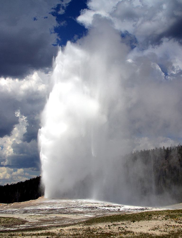
## We'll use data on the duration and spacing of eruptions
## of the old faithful geyser
## Data are eruption duration and waiting time to next eruption
data ("faithful") # load data
str (faithful) # display the internal structure of an R object
## 'data.frame': 272 obs. of 2 variables: ## $ eruptions: num 3.6 1.8 3.33 2.28 4.53 ... ## $ waiting : num 79 54 74 62 85 55 88 85 51 85 ...
Data summaries
A "statistic" is a the result of applying a function (summary) to the data: statistic <- function(data)
E.g. ranks: Min, Quantiles, Median, Mean, Max
summary (faithful$eruptions)
## Min. 1st Qu. Median Mean 3rd Qu. Max. ## 1.600 2.163 4.000 3.488 4.454 5.100
Roughly, a quantile for a proportion \(p\) is a value \(x\) for which \(p\) of the data are less than or equal to \(x\). The first quartile, median, and third quartile are the quantiles for \(p=0.25\), \(p=0.5\), and \(p=0.75\), respectively.
Visual Summary 1: Box Plot
boxplot (faithful$eruptions, main="Eruption time", horizontal=T)

Visual Summary 1.5: Box Plot, Jitter Plot
library(ggplot2);library(gridExtra); #boxplot relatives
b1<-ggplot(faithful, aes(x="All",y=eruptions)) + labs(x=NULL) + geom_boxplot()
#jitter plot
b2<-ggplot(faithful, aes(x="All",y=eruptions)) + labs(x=NULL) +
geom_jitter(position=position_jitter(height=0,width=0.25))
grid.arrange(b1, b2, nrow=1)

Visual Summary 2: Histogram
## Construct histogram of eruption times, plot data points on the x axis
hist (faithful$eruptions, main="Eruption time", xlab="Time (minutes)",
ylab="Count")
points (x=faithful$eruptions,y=rep(0,length(faithful$eruptions)), lwd=4, col='blue')

Visual Summary 2.5: Histogram
## Construct different histogram of eruption times ggplot(faithful, aes(x=eruptions)) + labs(y="Proportion") + geom_histogram(aes(y = ..count../sum(..count..)))

Replicates
- Common assumption is that data consists of replicates that are "the same."
- Come from "the same population"
- Come from "the same process"
- The goal of data analysis is to understand what the data tell us about the population.
Randomness
We often assume that we can treat items as if they were distributed "randomly."
- "That's so random!"
- Result of a coin flip is random
- Passengers were screened at random
- "random" does not mean "uniform"
- Mathematical formalism: events and probability
Sample Spaces and Events
- Sample space \({\mathcal{S}}\) is the set of all possible events we might observe. Depends on context.
- Coin flips: \({\mathcal{S}}= \{ h, t \}\)
- Eruption times: \({\mathcal{S}}= {\mathbb{R}}^{\ge 0}\)
- (Eruption times, Eruption waits): \({\mathcal{S}}= {\mathbb{R}}^{\ge 0} \times {\mathbb{R}}^{\ge 0}\)
- An event is a subset of the sample space.
- Observe heads: \(\{ h \}\)
- Observe eruption for 2 minutes: \(\{ 2.0 \}\)
- Observe eruption with length between 1 and 2 minutes and wait between 50 and 70 minutes: \([1,2] \times [50,70]\).
Event Probabilities
Any event can be assigned a probability between \(0\) and \(1\) (inclusive).
- \(\Pr(\{h\}) = 0.5\)
- \(\Pr([1,2] \times [50,70]) = 0.10\)
Interpreting probability:
Objectivist view
- Suppose we observe \(n\) replications of an experiment.
- Let \(n(A)\) be the number of times event \(A\) was observed
- \(\lim_{n \to \infty} \frac{n(A)}{n} = \Pr(A)\)
This is (loosely) Borel's Law of Large Numbers
Subjective interpretation is possible as well. ("Bayesian" statistics is related to this idea – more later.)
Abstraction of data: Random Variable
- We often reduce data to numbers.
- "\(1\) means heads, \(0\) means tails."
A random variable is a mapping from the event space to a number (or vector.)
Usually rendered in uppercase italics
\(X\) is every statistician's favourite, followed closely by \(Y\) and \(Z\).
"Realizations" of \(X\) are written in lower case, e.g. \(x_1\), \(x_2\), …
We will write the set of possible realizations as: \(\mathcal{X}\) for \(X\),
\(\mathcal{Y}\) for \(Y\), and so on.
Distributions of random variables
Realizations are observed according to probabilities specified by the distribution of \(X\)
Can think of \(X\) as an "infinite supply of data"
Separate realizations of the same r.v. \(X\) are "independent and identically distributed" (i.i.d.)
Formal definition of a random variable requires measure theory, not covered here
Probabilities for random variables
Random variable \(X\), realization \(x\).
- What is the probability we see \(x\)?
- \(\Pr(X=x)\), (if lazy, \(\Pr(x)\), but don't do this)
- Subsets of the domain of a random variable correspond to events.
- \(\Pr(X > 0)\) probability that I see a realization that is positive.
Discrete Random Variables
- Discrete random variables take values from a countable set
- Coin flip \(X\)
- \(\mathcal{X} = \{0,1\}\)
- Number of snowflakes that fall in a day \(Y\)
- \(\mathcal{Y} = \{0, 1, 2, ...\}\)
- Coin flip \(X\)
Probability Mass Function (PMF)
- For a discrete \(X\), \(p_{X}(x)\) gives \(\Pr(X = x)\).
- Requirement: \(\sum_{x \in \mathcal{X}} p_{X}(x) = 1\).
- Note that the sum can have an infinite number of terms.
Probability Mass Function (PMF) Example
\(X\) is number of "heads" in 20 flips of a fair coin
\(\mathcal{X} = \{0,1,...,20\}\)

Cumulative Distribution Function (CDF)
- For a discrete \(X\), \(P_{X}(x)\) gives \(\Pr(X \le x)\).
- Requirements:
- \(P\) is nondecreasing
- \(\sup_{x \in \mathcal{X}} P_{X}(x) = 1\)
- Note:
- \(P_X(b) = \sum_{x \le b} p_X(x)\)
- \(\Pr(a < X \le b) = P_X(b) - P_X(a)\)
Cumulative Distribution Function (CDF) Example
\(X\) is number of "heads" in 20 flips of a fair coin

Continuous random variables
- Continuous random variables take values in intervals of \({\mathbb{R}}\)
- Mass \(M\) of a star
- \(\mathcal{M} = (0,\infty)\)
- Oxygen saturation \(S\) of blood
- \(\mathcal{S} = [0,1]\)
- For a continuous r.v. \(X\), \(\Pr(X = x) = 0\) for all \(x\).
There is no probability mass function. - However, \(\Pr(X \in (a,b)) \ne 0\) in general.
Probability Density Function (PDF)
- For continuous \(X\), \(\Pr(X = x) = 0\) and PMF does not exist.
- However, we define the Probability Density Function \(f_X\):
- \(\Pr(a \le X \le b) = \int_{a}^{b} f_X(x) {\mathrm{\,d}}x\)
- Requirement:
- \(\forall x \;f_X(x) > 0\), \(\int_{-\infty}^\infty f_X(x) {\mathrm{\,d}}x = 1\)
Probability Density Function (PDF) Example

Cumulative Distribution Function (CDF)
- For a continuous \(X\), \(F_{X}(x)\) gives \(\Pr(X \le x) = \Pr(X \in (-\infty,x])\).
- Requirements:
- \(F\) is nondecreasing
- \(\sup_{x \in \mathcal{X}} F_{X}(x) = 1\)
- Note:
- \(F_X(x) = \int_{-\infty}^x f_X(x) {\mathrm{\,d}}x\)
- \(\Pr(x_1 < X \le x_2) = F_X(x_2) - F_X(x_1)\)
Cumulative Distribution Function (CDF) Example

Expectation
- The expected value of a discrete random variable \(X\) is denoted
\[{\mathrm{E}}[X] = \sum_{x \in \mathcal{X}} x \cdot p_X(X = x)\]
- The expected value of a continuous random variable \(Y\) is denoted
\[{\mathrm{E}}[Y] = \int_{y \in \mathcal{Y}} y \cdot f_Y(Y = y) {\mathrm{\,d}}y\]
- \({\mathrm{E}}[X]\) is called the mean of \(X\), often denoted \(\mu\) or \(\mu_X\).
Sample Mean
- Given a dataset (collection of realizations) \(x_1, x_2, ..., x_n\) of \(X\), the sample mean is:
\[ \bar{x}_n = \frac{1}{n} \sum_i x_i \]
Given a dataset, \(\bar x_n\) is a fixed number.
It is usually a good estimate of the expected value of a random variable \(X\) with an unknown distribution. (More on this later.)
Relationships between variables

- Random vectors or vector-valued random variables.
- Variables that occur together in some meaningful sense.
Joint distribution
\(X\) and \(Y\) have a joint distribution if their realizations come together as a pair. \((X,Y)\) is a random vector, and realizations may be written \((x_1,y_1), (x_2,y_2), ...\), or \(\langle x_1, y_1 \rangle, \langle x_2, y_2 \rangle, ...\)
faithful
Correlation (JWHT 2.3,3.1.3)
Pearson Correlation
\[ \rho_{X,Y} = \frac{E[(X - \mu_X)(Y - \mu_Y)]}{\sigma_X\sigma_Y} \]
Pearson Correlation: "Plugin" Estimate
\[ r_{X,Y} = \frac{\sum_{i=1}^n (x_i - \bar{x})(y_i - \bar{y})}{\sqrt{\sum_{i=1}^n (x_i - \bar{x})^2}\sqrt{\sum_{i=1}^n (y_i - \bar{y})^2}} \]
Sample Correlation
## eruptions waiting ## eruptions 1.0000000 0.9008112 ## waiting 0.9008112 1.0000000
Correlation Gotchas

Joint distribution - Density

Marginal distributions - Densities

Marginal distributions - Rug Plot

Conditional distributions

Conditional distributions

Conditional distributions

Conditional distributions

Conditional distributions

Conditional distributions

Conditional distributions

Conditional distributions

Independence
- Two random variables \(X\) and \(Y\) that are part of a random vector are independent iff:
\[ F_{X,Y}(x,y) = F_X(x)F_Y(y) \]
- Consequences:
\[ \Pr(X=x|Y=y) = \Pr(X=x) \]
\[ \Pr(Y=y|X=x) = \Pr(Y=y) \]
- Any conditional distribution of \(X\) is the same as the marginal distribution of \(X\)
- Knowing about \(Y\) provides no information about \(X\).
Independence vs. Correlation

## x y ## x 1.0000000 0.6996526 ## y 0.6996526 1.0000000
Independence vs. Correlation

## x y ## x 1.0000000000 0.0003411402 ## y 0.0003411402 1.0000000000
Independence vs. Correlation

## x y ## x 1.000000000 0.002031327 ## y 0.002031327 1.000000000
Independence vs. Correlation

## x y ## x 1.000000000 -0.008200447 ## y -0.008200447 1.000000000
Predicting Waiting Time

## Mean: 70.90
Conditional predictions
- If I know eruption time, can I do better?

## Mean: 55.60
Conditional predictions
- If I know eruption time, can I do better?

## Mean: 81.33
Conditional predictions?
- If I know eruption time, can I do better?
