---
title: "(Re)introduction to Statistics"
author: "Dan Lizotte"
date: "`r Sys.Date()`"
output:
pdf_document:
df_print: tibble
html_document:
df_print: paged
ioslides_presentation:
css: ../my_ioslides.css
df_print: paged
beamer_presentation: default
---
```{r echo=FALSE,warning=FALSE,message=FALSE}
library(ggplot2)
library(dplyr)
library(tibble)
```
## Recommended exercises
- JWHT 2.3 Lab: Introduction to R
(Or, follow along and see if you can do it in python.)
## Project {.smaller}
* I have a secret... ...your project might not work.
* That is okay. Prove to me and to your classmates that:
* You thoroughly understand the substantive area and problem
* You thoroughly understand the data
* You know what methods are reasonable to try and why
* You tried several ***and evaluated them rigorously***, but your predictions
are just not that good.
* You can’t get blood from a turnip. (But demonstrate that as best you can.)

## Model Choice
```{r echo=FALSE,warning=FALSE,message=FALSE,fig.width=8.5}
library(gridExtra)
ex <- data.frame(x0=rep(1,10),x=c(0.86,0.09,-0.85,0.87,-0.44,-0.43,-1.10,0.40,-0.96,0.17), y=c(2.49,0.83,-0.25,3.10,0.87,0.02,-0.12,1.81,-0.83,0.43))
form <- y ~ x; mod <- lm(form, data=ex); ex$pred <- predict(mod,ex)
fitplots_aes <- aes(x=x,y=y,xend=x,yend=pred)
pymin=-1;pymax=3.3
f1 <- ggplot(ex,fitplots_aes) + geom_point(size=4) + geom_smooth(method="lm",formula=form,se=F,n=200,na.rm=F) + coord_cartesian(ylim=c(pymin,pymax)) + geom_segment(color="red")
form <- y ~ x + I(x^2) + I(x^3) + I(x^4) + I(x^5) + I(x^6) + I(x^7) + I(x^8)
mod <- lm(form, data=ex); ex$pred <- predict(mod,ex)
f8 <- ggplot(ex,fitplots_aes) + geom_point(size=4) + geom_smooth(method="lm",formula=form,se=F,n=200,na.rm=F) + coord_cartesian(ylim=c(pymin,pymax)) + geom_segment(color="red")
grid.arrange(f1,f8,nrow=1)
```
## Model "Stability"
```{r echo=FALSE,fig.width=8.5,fig.height=6,warning=FALSE}
library(gridExtra)
ex.1 <- ex[-8,] # Remove 8th observation
form <- y ~ x; mod <- lm(form, data=ex.1); ex.1$pred <- predict(mod,ex.1)
f1.1 <- ggplot(ex.1,fitplots_aes) + geom_point(size=4) + geom_smooth(method="lm",formula=form,se=F,n=200,na.rm=F) + coord_cartesian(ylim=c(pymin,pymax)) + geom_segment(color="red")
form <- y ~ x + I(x^2) + I(x^3) + I(x^4) + I(x^5) + I(x^6) + I(x^7) + I(x^8)
mod <- lm(form, data=ex.1); ex.1$pred <- predict(mod,ex.1)
f8.1 <- ggplot(ex.1,fitplots_aes) + geom_point(size=4) + geom_smooth(method="lm",formula=form,se=F,n=200,na.rm=F) + coord_cartesian(ylim=c(pymin,pymax)) + geom_segment(color="red")
grid.arrange(f1,f8,f1.1,f8.1,nrow=2)
```
## Where did the data come from?
- One row is an observation. What does that mean?
- How are rows generated?
## Replicates
- Common assumption is that data consists of replicates that are "the same."
- Come from "the same population"
- Come from "the same process"
- The goal of data analysis is to understand what the data tell us about the population.
## Randomness
We often assume that we can treat items as if they were distributed "*randomly*."
- "*That's so random!*"
- Result of a coin flip is "random"
- Passengers were screened "at random"
>- "random" does not mean "uniform"
>- Mathematical formalism: _events_ and _probability_
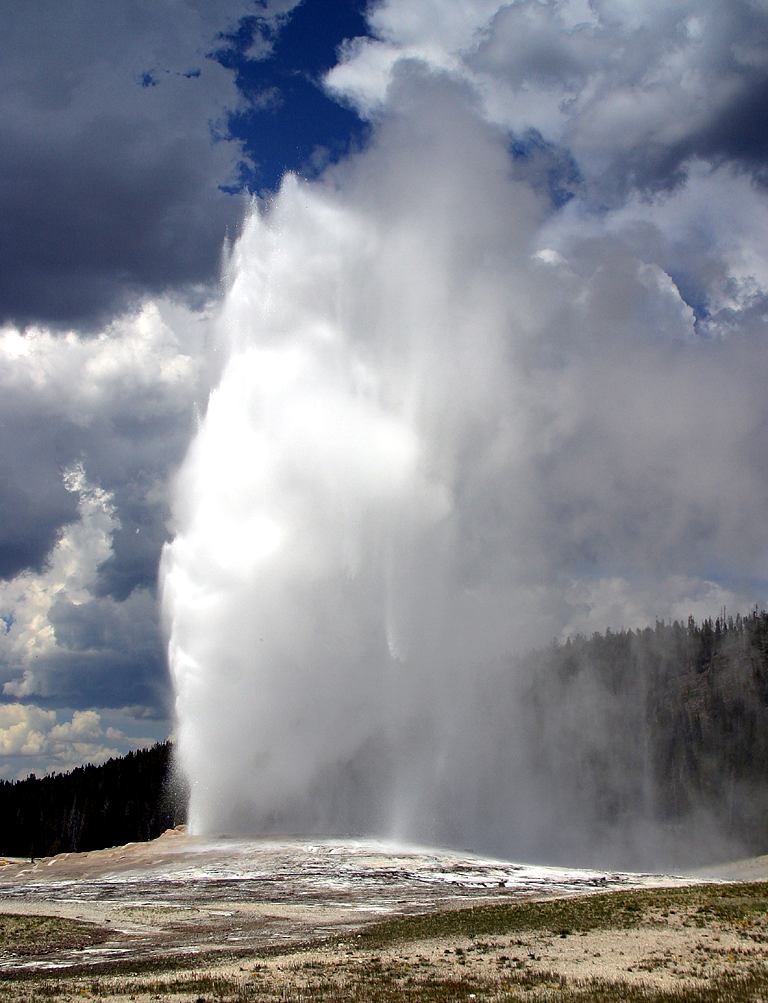
## Example Scenario - Old Faithful
```{r rows.print=15,echo=FALSE}
## As an example, we'll use measurements on the duration and spacing of eruptions
## of the old faithful geyser
## Measurements are eruption duration and waiting time to next eruption
data ("faithful") # load data
faithful
```
 ## Sample Spaces and Events
\newcommand{\Samp}{\mathcal{S}}
\renewcommand{\Re}{\mathbb{R}}
- _Sample space_ $\Samp$ is the set of all possible events we might observe. Depends on context.
- Coin flips: $\Samp = \{ h, t \}$
- Eruption times: $\Samp = \Re^{\ge 0}$
- (Eruption times, Eruption waits): $\Samp = \Re^{\ge 0} \times \Re^{\ge 0}$
- An _event_ is a subset of the sample space.
- Observe heads: $\{ h \}$
- Observe eruption for 2 minutes: $\{ 2.0 \}$
- Observe eruption with length between 1 and 2 minutes and wait between 50 and 70 minutes: $[1,2] \times [50,70]$.
## Event Probabilities
Any event can be assigned a _probability_ between $0$ and $1$ (inclusive).
- $\Pr(\{h\}) = 0.5$
- $\Pr([1,2] \times [50,70]) = 0.10$
Probability of the observation falling *somewhere* in the sample space is 1.0.
- $\Pr(\Samp) = 1$
## Interpreting probability:
## Sample Spaces and Events
\newcommand{\Samp}{\mathcal{S}}
\renewcommand{\Re}{\mathbb{R}}
- _Sample space_ $\Samp$ is the set of all possible events we might observe. Depends on context.
- Coin flips: $\Samp = \{ h, t \}$
- Eruption times: $\Samp = \Re^{\ge 0}$
- (Eruption times, Eruption waits): $\Samp = \Re^{\ge 0} \times \Re^{\ge 0}$
- An _event_ is a subset of the sample space.
- Observe heads: $\{ h \}$
- Observe eruption for 2 minutes: $\{ 2.0 \}$
- Observe eruption with length between 1 and 2 minutes and wait between 50 and 70 minutes: $[1,2] \times [50,70]$.
## Event Probabilities
Any event can be assigned a _probability_ between $0$ and $1$ (inclusive).
- $\Pr(\{h\}) = 0.5$
- $\Pr([1,2] \times [50,70]) = 0.10$
Probability of the observation falling *somewhere* in the sample space is 1.0.
- $\Pr(\Samp) = 1$
## Interpreting probability:
Objectivist view
- Suppose we observe $n$ replications of an experiment.
- Let $n(A)$ be the number of times event $A$ was observed
- $\lim_{n \to \infty} \frac{n(A)}{n} = \Pr(A)$
- This is (loosely) *Borel's Law of Large Numbers*
- Subjective interpretation is possible as well. ("Bayesian" statistics is related to this idea -- more later.)
## Abstraction of data-generating process: Random Variable
- We often reduce data to numbers.
- "$1$ means heads, $0$ means tails."
- A _random variable_ is a mapping from the event space to a number (or vector.)
- Usually rendered in uppercase *italics*
- $X$ is every statistician's favourite, followed closely by $Y$ and $Z$.
- "Realizations" of $X$ are written in lower case, e.g. $x_1$, $x_2$, ...
- We will write the set of possible realizations as: $\mathcal{X}$ for $X$,
$\mathcal{Y}$ for $Y$, and so on.
## Distributions of random variables
- Realizations are observed according to probabilities specified by the *distribution* of $X$
- Can think of $X$ as an "infinite supply of data"
- Separate realizations of the same r.v. $X$ are "independent and identically distributed" (i.i.d.)
- Formal definition of a random variable requires measure theory, not covered here
## Probabilities for random variables
Random variable $X$, realization $x$.
- What is the probability we see $x$?
- $\Pr(X=x)$, (if lazy, $\Pr(x)$, but don't do this)
- Subsets of the domain of a random variable correspond to events.
- $\Pr(X > 0)$ probability that I see a realization that is positive.
## Discrete Random Variables
- Discrete random variables take values from a countable set
- Coin flip $X$
- $\mathcal{X} = \{0,1\}$
- Number of snowflakes that fall in a day $Y$
- $\mathcal{Y} = \{0, 1, 2, ...\}$
## Probability Mass Function (PMF)
- For a discrete $X$, $p_{X}(x)$ gives $\Pr(X = x)$.
- Requirement: $\sum_{x \in \mathcal{X}} p_{X}(x) = 1$.
- Note that the sum can have an infinite number of terms.
## Probability Mass Function (PMF) Example
$X$ is number of "heads" in 20 flips of a fair coin
$\mathcal{X} = \{0,1,...,20\}$
```{r echo=F}
pmfData <- data.frame( x = 0:20, px = dbinom(0:20, 20, .5)); eps = 0.05;
ggplot(pmfData,aes(x = x,y = px,ymin=0,ymax=px)) + geom_point(size=3) +
geom_segment(x = pmfData$x + eps, xend=(pmfData$x + 1 - eps),y = 0, yend = 0) + geom_point(y = 0, size=3, shape=1) +
ylab(expression(p[X](x))) + scale_x_continuous(breaks=seq(0,20,5))
```
## Cumulative Distribution Function (CDF)
- For a discrete $X$, $P_{X}(x)$ gives $\Pr(X \le x)$.
- Requirements:
- $P$ is nondecreasing
- $\sup_{x \in \mathcal{X}} P_{X}(x) = 1$
- Note:
- $P_X(b) = \sum_{x \le b} p_X(x)$
- $\Pr(a < X \le b) = P_X(b) - P_X(a)$
## Cumulative Distribution Function (CDF) Example
$X$ is number of "heads" in 20 flips of a fair coin
```{r echo=F}
cdfData <- data.frame(x = 0:20, px = pbinom(0:20, 20, .5))
ggplot(cdfData,aes(x=x,y=px,ymin=0,ymax=px)) +
geom_segment(xend=(cdfData$x + 1),yend = cdfData$px) +
geom_point(size=3) + geom_point(x=(cdfData$x+1), size=3, shape=1) +
ylab(expression(P[X](x))) + scale_x_continuous(breaks=seq(0,20,5))
```
## Continuous random variables
- Continuous random variables take values in intervals of $\Re$
- Mass $M$ of a star
- $\mathcal{M} = (0,\infty)$
- Oxygen saturation $S$ of blood
- $\mathcal{S} = [0,1]$
- For a continuous r.v.\ $X$, $\Pr(X = x) = 0$ for all $x$.
***There is no probability mass function.***
- However, $\Pr(X \in (a,b)) \ne 0$ in general.
## Probability Density Function (PDF)
\newcommand{\diff}{\mathrm{\,d}}
- For continuous $X$, $\Pr(X = x) = 0$ and PMF does not exist.
- However, we define the *Probability Density Function* $f_X$:
- $\Pr(a \le X \le b) = \int_{a}^{b} f_X(x) \diff x$
- Requirement:
- $\forall x \;f_X(x) > 0$, $\int_{-\infty}^\infty f_X(x) \diff x = 1$
## Probability Density Function (PDF) Example
```{r echo=F}
ggplot(data.frame(x = c(0, 20)), aes(x)) + ylab("Density") +
stat_function(fun = function(x){dchisq(x,5)}, colour = "black")
```
## Cumulative Distribution Function (CDF)
- For a continuous $X$, $F_{X}(x)$ gives $\Pr(X \le x) = \Pr(X \in (-\infty,x])$.
- Requirements:
- $F$ is nondecreasing
- $\sup_{x \in \mathcal{X}} F_{X}(x) = 1$
- Note:
- $F_X(x) = \int_{-\infty}^x f_X(x) \diff x$
- $\Pr(x_1 < X \le x_2) = F_X(x_2) - F_X(x_1)$
## Cumulative Distribution Function (CDF) Example
```{r echo=F}
ggplot(data.frame(x = c(0, 20)), aes(x)) + ylab("Probability") +
stat_function(fun = function(x){pchisq(x,5)}, colour = "black")
```
## Joint Distributions
Two random variables $X$ and $Y$ have a **joint distribution** if their realizations come together as a pair. $(X,Y)$ is a **random vector**, and realizations may be written $(x_1,y_1), (x_2,y_2), ...$, or $\langle x_1, y_1 \rangle, \langle x_2, y_2 \rangle, ...$
- Joint Cumulative Distribution Function (CDF)
- We define the *Joint Cumulative Distribution Function* $F_{X,Y}$:
- $\Pr(X \le b, Y \le d) = F_{X,Y}(b,d)$
- Joint Probability Density Function (PDF)
- We define the *Joint Probability Density Function* $f_{X,Y}$:
- $\Pr(\langle X , Y \rangle \in \mathcal{R} \subseteq \mathcal{X} \times \mathcal{Y}) = \int_{\mathcal{R}} f_{X,Y}(x,y) \diff x \diff y$
## Joint Density
```{r echo=F}
fbase <- ggplot(data=faithful,aes(x=eruptions,y=waiting)) + xlim(1,5.75) + ylim(38,100) + scale_fill_distiller(palette="Greys",direction=1) + theme(legend.position="none")
fbase + stat_density_2d(geom="polygon",aes(fill = ..level..)) #+ geom_point(alpha=I(1/4))
```
## Supervised Learning Framework
(JWHT 2, HTF 2)
Training set: a set of ***labeled examples*** of the form
\[\langle x_1,\,x_2,\,\dots x_p,y\rangle,\]
where $x_j$ are ***feature values*** and $y$ is the ***output***
* Task: ***Given a new $x_1,\,x_2,\,\dots x_p$, predict $y$***
What to learn: A ***function*** $h:\mathcal{X}_1 \times \mathcal{X}_2 \times \cdots \times
\mathcal{X}_p \rightarrow \mathcal{Y}$, which maps the features into the output
domain
* Goal: Make accurate ***future predictions*** (on unseen data)
## Common Assumptions
- Data are realizations of a random variable $(X_1, X_2, ..., Y)$
- Future data will be realizations of the same random variable
- We are given a **loss function** $\ell$ which measures how happy we are with our prediction $\hat{y}$ if the true observation is $(x,y)$.
- $\ell(\hat{y}, y)$ is non-negative, and the worse the prediction, the larger it is.
## Great Expectations
\newcommand{\E}{\mathrm{E}}
- The _expected value_ of a discrete random variable $X$ is denoted
$$\E[X] = \sum_{x \in \mathcal{X}} x \cdot p_X(X = x)$$
- The _expected value_ of a continuous random variable $Y$ is denoted
$$\E[Y] = \int_{y \in \mathcal{Y}} y \cdot f_Y(Y = y) \diff y$$
- $\E[X]$ is called the **mean** of $X$, often denoted $\mu$ or $\mu_X$.
## Sample Mean
- Given a ***dataset*** (collection of realizations) $x_1, x_2, ..., x_n$ of $X$, the **sample mean** is:
$$ \bar{x}_n = \frac{1}{n} \sum_i x_i $$
Given a dataset, $\bar x_n$ is a fixed number.
It is usually a good estimate of the expected value of a random variable $X$ with an unknown distribution. (More on this later.)
## Generalization Error
- Suppose we are given a function $h$ to use for predictions
- If $X$ is a random variable, then so is $h(X)$
- And, so is $\ell(h(X),Y)$
Under the assumption that future data are produced by a random variable $(X,Y)$, the ***expected loss*** of a given classifier is
$$
E[\ell(h(X),Y)]
$$
## Test Error
- Given a ***dataset*** (collection of realizations) $(x_1, y_1), (x_2, y_2), ..., (x_n, y_n)$ of $(X,Y)$, ***that were not used to find $h$*** the **test error** is:
$$ \bar{\ell}_{h,n} = \frac{1}{n} \sum_i \ell(h(x_i),y_i) $$
Given a test dataset, $\bar \ell_n$ is a fixed number.
It has all the properties of a sample mean, which we will discuss.
## Model Choice
Which one do you think has the best Generalization Error? Why?
```{r echo=FALSE,warning=FALSE,message=FALSE,fig.width=8.5}
library(gridExtra)
ex <- data.frame(x0=rep(1,10),x=c(0.86,0.09,-0.85,0.87,-0.44,-0.43,-1.10,0.40,-0.96,0.17), y=c(2.49,0.83,-0.25,3.10,0.87,0.02,-0.12,1.81,-0.83,0.43))
form <- y ~ x; mod <- lm(form, data=ex); ex$pred <- predict(mod,ex)
fitplots_aes <- aes(x=x,y=y,xend=x,yend=pred)
pymin=-1;pymax=3.3
f1 <- ggplot(ex,fitplots_aes) + geom_point(size=4) + geom_smooth(method="lm",formula=form,se=F,n=200,na.rm=F) + coord_cartesian(ylim=c(pymin,pymax)) + geom_segment(color="red")
form <- y ~ x + I(x^2) + I(x^3) + I(x^4) + I(x^5) + I(x^6) + I(x^7) + I(x^8) + I(x^9)
mod <- lm(form, data=ex); ex$pred <- predict(mod,ex)
f8 <- ggplot(ex,fitplots_aes) + geom_point(size=4) + geom_smooth(method="lm",formula=form,se=F,n=200,na.rm=F) + coord_cartesian(ylim=c(pymin,pymax)) + geom_segment(color="red")
grid.arrange(f1,f8,nrow=1)
```