2018-09-20

Recommended exercises

Project

  • I have a secret… …your project might not work.
  • That is okay. Prove to me and to your classmates that:
    • You thoroughly understand the substantive area and problem
    • You thoroughly understand the data
    • You know what methods are reasonable to try and why
    • You tried several and evaluated them rigorously, but your predictions are just not that good.
  • You can’t get blood from a turnip. (But demonstrate that as best you can.)

Model Choice

Model “Stability”

Where did the data come from?

  • One row is an observation. What does that mean?
  • How are rows generated?

Replicates

  • Common assumption is that data consists of replicates that are “the same.”
  • Come from “the same population”
  • Come from “the same process”
  • The goal of data analysis is to understand what the data tell us about the population.

Randomness

We often assume that we can treat items as if they were distributed “randomly.”
  • That’s so random!
  • Result of a coin flip is “random”
  • Passengers were screened “at random”
  • “random” does not mean “uniform”
  • Mathematical formalism: events and probability

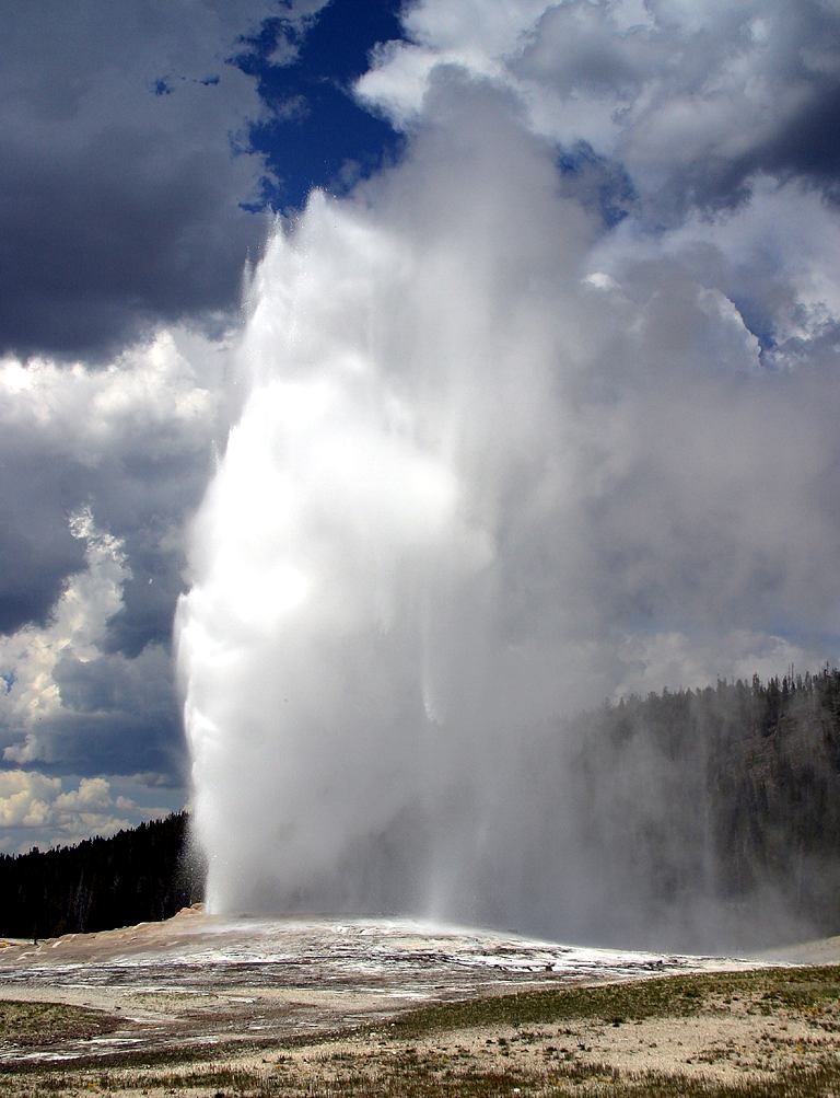
Example Scenario - Old Faithful

Old Faithfull-pdPhoto by Jon Sullivan

Sample Spaces and Events

  • Sample space \(\mathcal{S}\) is the set of all possible events we might observe. Depends on context.
    • Coin flips: \(\mathcal{S}= \{ h, t \}\)
    • Eruption times: \(\mathcal{S}= \mathbb{R}^{\ge 0}\)
    • (Eruption times, Eruption waits): \(\mathcal{S}= \mathbb{R}^{\ge 0} \times \mathbb{R}^{\ge 0}\)
  • An event is a subset of the sample space.
    • Observe heads: \(\{ h \}\)
    • Observe eruption for 2 minutes: \(\{ 2.0 \}\)
    • Observe eruption with length between 1 and 2 minutes and wait between 50 and 70 minutes: \([1,2] \times [50,70]\).

Event Probabilities

Any event can be assigned a probability between \(0\) and \(1\) (inclusive).

  • \(\Pr(\{h\}) = 0.5\)
  • \(\Pr([1,2] \times [50,70]) = 0.10\)

Probability of the observation falling somewhere in the sample space is 1.0.

  • \(\Pr(\mathcal{S}) = 1\)

Interpreting probability:
Objectivist view

  • Suppose we observe \(n\) replications of an experiment.
  • Let \(n(A)\) be the number of times event \(A\) was observed
  • \(\lim_{n \to \infty} \frac{n(A)}{n} = \Pr(A)\)
  • This is (loosely) Borel’s Law of Large Numbers

  • Subjective interpretation is possible as well. (“Bayesian” statistics is related to this idea – more later.)

Abstraction of data-generating process: Random Variable

  • We often reduce data to numbers.
    • “\(1\) means heads, \(0\) means tails.”
  • A random variable is a mapping from the event space to a number (or vector.)

  • Usually rendered in uppercase italics

  • \(X\) is every statistician’s favourite, followed closely by \(Y\) and \(Z\).

  • “Realizations” of \(X\) are written in lower case, e.g. \(x_1\), \(x_2\), …

  • We will write the set of possible realizations as: \(\mathcal{X}\) for \(X\), \(\mathcal{Y}\) for \(Y\), and so on.

Distributions of random variables

  • Realizations are observed according to probabilities specified by the distribution of \(X\)

  • Can think of \(X\) as an “infinite supply of data”

  • Separate realizations of the same r.v. \(X\) are “independent and identically distributed” (i.i.d.)

  • Formal definition of a random variable requires measure theory, not covered here

Probabilities for random variables

Random variable \(X\), realization \(x\).

  • What is the probability we see \(x\)?
    • \(\Pr(X=x)\), (if lazy, \(\Pr(x)\), but don’t do this)
  • Subsets of the domain of a random variable correspond to events.
    • \(\Pr(X > 0)\) probability that I see a realization that is positive.

Discrete Random Variables

  • Discrete random variables take values from a countable set
    • Coin flip \(X\)
      • \(\mathcal{X} = \{0,1\}\)
    • Number of snowflakes that fall in a day \(Y\)
      • \(\mathcal{Y} = \{0, 1, 2, ...\}\)

Probability Mass Function (PMF)

  • For a discrete \(X\), \(p_{X}(x)\) gives \(\Pr(X = x)\).
  • Requirement: \(\sum_{x \in \mathcal{X}} p_{X}(x) = 1\).
    • Note that the sum can have an infinite number of terms.

Probability Mass Function (PMF) Example

\(X\) is number of “heads” in 20 flips of a fair coin
\(\mathcal{X} = \{0,1,...,20\}\)

Cumulative Distribution Function (CDF)

  • For a discrete \(X\), \(P_{X}(x)\) gives \(\Pr(X \le x)\).
  • Requirements:
    • \(P\) is nondecreasing
    • \(\sup_{x \in \mathcal{X}} P_{X}(x) = 1\)
  • Note:
    • \(P_X(b) = \sum_{x \le b} p_X(x)\)
    • \(\Pr(a < X \le b) = P_X(b) - P_X(a)\)

Cumulative Distribution Function (CDF) Example

\(X\) is number of “heads” in 20 flips of a fair coin

Continuous random variables

  • Continuous random variables take values in intervals of \(\mathbb{R}\)
  • Mass \(M\) of a star
    • \(\mathcal{M} = (0,\infty)\)
  • Oxygen saturation \(S\) of blood
    • \(\mathcal{S} = [0,1]\)


  • For a continuous r.v. \(X\), \(\Pr(X = x) = 0\) for all \(x\).
    There is no probability mass function.
  • However, \(\Pr(X \in (a,b)) \ne 0\) in general.

Probability Density Function (PDF)

  • For continuous \(X\), \(\Pr(X = x) = 0\) and PMF does not exist.
  • However, we define the Probability Density Function \(f_X\):
    • \(\Pr(a \le X \le b) = \int_{a}^{b} f_X(x) \mathrm{\,d}x\)
  • Requirement:
    • \(\forall x \;f_X(x) > 0\), \(\int_{-\infty}^\infty f_X(x) \mathrm{\,d}x = 1\)

Probability Density Function (PDF) Example

Cumulative Distribution Function (CDF)

  • For a continuous \(X\), \(F_{X}(x)\) gives \(\Pr(X \le x) = \Pr(X \in (-\infty,x])\).
  • Requirements:
    • \(F\) is nondecreasing
    • \(\sup_{x \in \mathcal{X}} F_{X}(x) = 1\)
  • Note:
    • \(F_X(x) = \int_{-\infty}^x f_X(x) \mathrm{\,d}x\)
    • \(\Pr(x_1 < X \le x_2) = F_X(x_2) - F_X(x_1)\)

Cumulative Distribution Function (CDF) Example

Joint Distributions

Two random variables \(X\) and \(Y\) have a joint distribution if their realizations come together as a pair. \((X,Y)\) is a random vector, and realizations may be written \((x_1,y_1), (x_2,y_2), ...\), or \(\langle x_1, y_1 \rangle, \langle x_2, y_2 \rangle, ...\)

  • Joint Cumulative Distribution Function (CDF)
    • We define the Joint Cumulative Distribution Function \(F_{X,Y}\):
      • \(\Pr(X \le b, Y \le d) = F_{X,Y}(b,d)\)
  • Joint Probability Density Function (PDF)
    • We define the Joint Probability Density Function \(f_{X,Y}\):
      • \(\Pr(\langle X , Y \rangle \in \mathcal{R} \subseteq \mathcal{X} \times \mathcal{Y}) = \int_{\mathcal{R}} f_{X,Y}(x,y) \mathrm{\,d}x \mathrm{\,d}y\)


Joint Density

Supervised Learning Framework
(JWHT 2, HTF 2)

Training set: a set of labeled examples of the form

\[\langle x_1,\,x_2,\,\dots x_p,y\rangle,\]

where \(x_j\) are feature values and \(y\) is the output

  • Task: Given a new \(x_1,\,x_2,\,\dots x_p\), predict \(y\)

What to learn: A function \(h:\mathcal{X}_1 \times \mathcal{X}_2 \times \cdots \times \mathcal{X}_p \rightarrow \mathcal{Y}\), which maps the features into the output domain

  • Goal: Make accurate future predictions (on unseen data)

Common Assumptions

  • Data are realizations of a random variable \((X_1, X_2, ..., Y)\)

  • Future data will be realizations of the same random variable

  • We are given a loss function \(\ell\) which measures how happy we are with our prediction \(\hat{y}\) if the true observation is \((x,y)\).

  • \(\ell(\hat{y}, y)\) is non-negative, and the worse the prediction, the larger it is.

Great Expectations

  • The expected value of a discrete random variable \(X\) is denoted

\[\mathrm{E}[X] = \sum_{x \in \mathcal{X}} x \cdot p_X(X = x)\]

  • The expected value of a continuous random variable \(Y\) is denoted

\[\mathrm{E}[Y] = \int_{y \in \mathcal{Y}} y \cdot f_Y(Y = y) \mathrm{\,d}y\]

  • \(\mathrm{E}[X]\) is called the mean of \(X\), often denoted \(\mu\) or \(\mu_X\).

Sample Mean

  • Given a dataset (collection of realizations) \(x_1, x_2, ..., x_n\) of \(X\), the sample mean is:

\[ \bar{x}_n = \frac{1}{n} \sum_i x_i \]

Given a dataset, \(\bar x_n\) is a fixed number.

It is usually a good estimate of the expected value of a random variable \(X\) with an unknown distribution. (More on this later.)

Generalization Error

  • Suppose we are given a function \(h\) to use for predictions
  • If \(X\) is a random variable, then so is \(h(X)\)
  • And, so is \(\ell(h(X),Y)\)

Under the assumption that future data are produced by a random variable \((X,Y)\), the expected loss of a given classifier is

\[ E[\ell(h(X),Y)] \]

Test Error

  • Given a dataset (collection of realizations) \((x_1, y_1), (x_2, y_2), ..., (x_n, y_n)\) of \((X,Y)\), that were not used to find \(h\) the test error is:

\[ \bar{\ell}_{h,n} = \frac{1}{n} \sum_i \ell(h(x_i),y_i) \]

Given a test dataset, \(\bar \ell_n\) is a fixed number.

It has all the properties of a sample mean, which we will discuss.

Model Choice

Which one do you think has the best Generalization Error? Why?