---
title: "Supervised Learning"
author: "Dan Lizotte"
date: '`r Sys.Date()`'
output:
ioslides_presentation:
css: ../my_ioslides.css
html_document: default
pdf_document: null
---
```{r echo=F,message=F,warning=F}
library(dplyr)
library(gridExtra)
```
## Relationships between variables {.smaller}
```{r message=F,warning=F,echo=F}
library(ggplot2)
fbase <- ggplot(data=faithful,aes(x=eruptions,y=waiting)) + xlim(1,5.75) + ylim(38,100) + scale_fill_distiller(palette="Greys",direction=1) + theme(legend.position="none")
fbase + geom_point()
```
- ***Random vectors*** or ***vector-valued*** random variables.
- Variables that occur ***together*** in some meaningful sense.
## Joint distribution {.smaller}
```{r}
library(knitr);
kable(head(faithful,10))
```
## Correlation (JWHT 2.3,3.1.3)
```{r message=F,warning=F,echo=F}
library(ggplot2)
fbase <- ggplot(data=faithful,aes(x=eruptions,y=waiting)) + xlim(1,5.75) + ylim(38,100) + scale_fill_distiller(palette="Greys",direction=1) + theme(legend.position="none")
fbase + geom_point()
```
## Pearson Correlation
\[
\rho_{X,Y} = \frac{E[(X - \mu_X)(Y - \mu_Y)]}{\sigma_X\sigma_Y}
\]
## Pearson Correlation: "Plugin" Estimate
\[
r_{X,Y} = \frac{\sum_{i=1}^n (x_i - \bar{x})(y_i - \bar{y})}{\sqrt{\sum_{i=1}^n (x_i - \bar{x})^2}\sqrt{\sum_{i=1}^n (y_i - \bar{y})^2}}
\]
## Sample Correlation
```{r message=F,warning=F,echo=F}
library(ggplot2)
fbase <- ggplot(data=faithful,aes(x=eruptions,y=waiting)) + xlim(1,5.75) + ylim(38,100) + scale_fill_distiller(palette="Greys",direction=1) + theme(legend.position="none")
fbase + geom_point()
cor(faithful)
```
## Correlation Gotchas
## Joint distribution - Density {.smaller}
```{r echo=F}
fbase + stat_density_2d(geom="polygon",aes(fill = ..level..)) + geom_point(alpha=I(1/4))
```
## Marginal distributions - Densities
```{r echo=F}
mhist <- fbase + stat_density_2d(geom="polygon",aes(fill = ..level..)) + geom_point(alpha=I(1/4))
ggExtra::ggMarginal(mhist, type = "density")
```
## Marginal distributions - Rug Plot
```{r echo=F}
library(ggExtra)
fbase + stat_density_2d(geom="polygon",aes(fill = ..level..)) + geom_point(alpha=I(1/4)) + geom_rug(alpha=I(1/4),size=2)
```
## Conditional distributions
```{r echo=F}
cond1 = 60;
fbase + stat_density_2d(geom="polygon",aes(fill = ..level..)) + geom_point(alpha=I(1/4)) + geom_rug(alpha=I(1/4),size=2) + geom_hline(yintercept = I(cond1),color="blue")
```
## Conditional distributions
```{r echo=F}
ggplot(faithful %>% filter(waiting==cond1),aes(x=eruptions)) + geom_density() + xlim(1,5.75) +
ggtitle(paste0("f(eruptions|waiting=",cond1,")"))
```
## Conditional distributions
```{r echo=F}
cond2=80
fbase + stat_density_2d(geom="polygon",aes(fill = ..level..)) + geom_point(alpha=I(1/4)) + geom_rug(alpha=I(1/4),size=2) + geom_hline(yintercept = I(cond2),color="blue")
```
## Conditional distributions
```{r echo=F}
ggplot(faithful %>% filter(waiting==cond2),aes(x=eruptions)) + geom_density() + xlim(1,5.75) + ggtitle(paste0("f(eruptions|waiting=",cond2,")"))
```
## Conditional distributions
```{r echo=F}
cond3=c(2.0,2.1)
fbase + stat_density_2d(geom="polygon",aes(fill = ..level..)) + geom_point(alpha=I(1/4)) + geom_rug(alpha=I(1/4),size=2) + annotate("rect",xmin=cond3[1],xmax=cond3[2],ymin=-Inf,ymax=Inf,alpha=1/4,fill="blue")
```
## Conditional distributions
```{r echo=F}
ggplot(faithful %>% filter(cond3[1] <= eruptions, eruptions <= cond3[2]),aes(x=waiting)) + geom_density() + xlim(40,100) + ggtitle(paste0("f( waiting | ", cond3[1], " <= eruptions <= ",cond3[2],")")) + coord_flip()
```
## Conditional distributions
```{r echo=F}
cond4=c(4.4,4.5)
fbase + stat_density_2d(geom="polygon",aes(fill = ..level..)) + geom_point(alpha=I(1/4)) + geom_rug(alpha=I(1/4),size=2) + annotate("rect",xmin=cond4[1],xmax=cond4[2],ymin=-Inf,ymax=Inf,alpha=1/4,fill="blue")
```
## Conditional distributions
```{r echo=F}
ggplot(faithful %>% filter(cond4[1] <= eruptions, eruptions <= cond4[2]),aes(x=waiting)) + geom_density() + xlim(40,100) + ggtitle(paste0("f( waiting | ", cond4[1], " <= eruptions <= ",cond4[2],")")) + coord_flip()
```
## Independence
- Two random variables $X$ and $Y$ that are part of a random vector are **independent** iff:
\[
F_{X,Y}(x,y) = F_X(x)F_Y(y)
\]
- Consequences:
\[
\Pr(X=x|Y=y) = \Pr(X=x)
\]
\[
\Pr(Y=y|X=x) = \Pr(Y=y)
\]
- Any conditional distribution of $X$ is the same as the marginal distribution of $X$
- Knowing about $Y$ provides no information about $X$.
## Independence vs. Correlation
```{r echo=F,message=F,warning=F}
library(MASS);n=10000;mu <- c(0,0);Sig <- matrix(c(1,0.7,0.7,1),2,2);
xx <- mvrnorm(n,mu,Sig)
d <- data.frame(x=xx[,1],y=xx[,2])
ggplot(d,aes(x=x,y=y)) + geom_point(alpha=I(1/4)) + geom_rug()
cor(d)
```
## Independence vs. Correlation
```{r echo=F}
n=10000
x <- 2*pi*runif(n) - 2*pi
d <- data.frame(x=x,y=cos(x)+0.25*rnorm(n))
ggplot(d,aes(x=x,y=y)) + geom_point(alpha=I(1/4)) + geom_rug()
cor(d)
```
## Independence vs. Correlation
```{r echo=F}
n=10000
r <- runif(n)
theta <- runif(n)*2*pi
d <- data.frame(x=sqrt(r)*cos(theta),y=sqrt(r)*sin(theta))
ggplot(d,aes(x=x,y=y)) + geom_point(alpha=I(1/4)) + geom_rug()
cor(d)
```
## Independence vs. Correlation
```{r echo=F}
n=10000
d <- data.frame(x=rnorm(n),y=rnorm(n))
ggplot(d,aes(x=x,y=y)) + geom_point(alpha=I(1/4)) + geom_rug()
cor(d)
```
## Predicting Waiting Time
```{r echo=F}
pred <- mean(faithful$waiting)
ggplot(faithful,aes(x=waiting)) + geom_density() + xlim(40,100) + ggtitle(paste0("f( waiting | ", cond3[1], " <= eruptions <= ",cond3[2],")")) + geom_vline(xintercept=pred,color="red") + coord_flip()
message(sprintf("Mean: %.2f",pred))
```
## Conditional predictions
- If I know eruption time, can I do better?
```{r echo=F}
pred <- mean(subset(faithful,cond3[1] <= eruptions & eruptions <= cond3[2])$waiting)
ggplot(faithful %>% filter(cond3[1] <= eruptions, eruptions <= cond3[2]),aes(x=waiting)) + geom_density() + xlim(40,100) + ggtitle(paste0("f( waiting | ", cond3[1], " <= eruptions <= ",cond3[2],")")) + geom_vline(xintercept=pred,color="red") + coord_flip()
message(sprintf("Mean: %.2f",pred))
```
## Conditional predictions
- If I know eruption time, can I do better?
```{r echo=F}
pred <- mean(subset(faithful,cond4[1] <= eruptions & eruptions <= cond4[2])$waiting)
ggplot(faithful %>% filter(cond4[1] <= eruptions, eruptions <= cond4[2]),aes(x=waiting)) + geom_density() + xlim(40,100) + ggtitle(paste0("f( waiting | ", cond4[1], " <= eruptions <= ",cond4[2],")")) + geom_vline(xintercept=pred,color="red") + coord_flip()
message(sprintf("Mean: %.2f",pred))
```
## Conditional predictions?
- If I know eruption time, can I do better?
```{r echo=F}
cond5=c(3.15,3.25)
fbase + stat_density_2d(geom="polygon",aes(fill = ..level..)) + geom_point(alpha=I(1/4)) + geom_rug(alpha=I(1/4),size=2) + annotate("rect",xmin=cond5[1],xmax=cond5[2],ymin=-Inf,ymax=Inf,alpha=1/4,fill="blue")
```
## Supervised Learning Framework (HTF 2, JWHT 2)
Training experience: a set of ***labeled examples*** of the form
\[\langle x_1,\,x_2,\,\dots x_p,y\rangle,\]
where $x_j$ are ***feature values*** and $y$ is the ***output***
* Task: ***Given a new $x_1,\,x_2,\,\dots x_p$, predict $y$***
What to learn: A ***function*** $f:\mathcal{X}_1 \times \mathcal{X}_2 \times \cdots \times
\mathcal{X}_p \rightarrow \mathcal{Y}$, which maps the features into the output
domain
* Goal: Make accurate ***future predictions*** (on unseen data)
* Plan: Learn to make accurate predictions on the training data
## [Wisconsin Breast Cancer Prognostic Data](http://archive.ics.uci.edu/ml/datasets/Breast+Cancer+Wisconsin+(Prognostic)) {.smaller}
```{r echo=F}
#setwd("/Users/dlizotte/Seafile/My Library/Teaching/cs4437/Lectures/5_Supervised Learning")
wpbc_featurenames = c("Radius","Texture","Perimeter","Area","Smoothness","Compactness","Concavity","Concave Points","Symmetry","Fractal Dim")
wpbc_names = c("ID","Outcome","Time",paste(wpbc_featurenames,"Mean"),paste(wpbc_featurenames,"SE"),paste(wpbc_featurenames,"Worst"),"Tumor Diameter","Lymph Status")
bc <- read.csv("data/wpbc.data.txt",header=FALSE,col.names=wpbc_names)
```
Cell samples were taken from tumors in breast cancer patients before
surgery and imaged; tumors were excised; patients were followed to determine whether or not the cancer
recurred, and how long until recurrence or disease free.
![image](images/xcyt1.gif)
## Wisconsin data (continued) {.smaller}
- 198 instances, 32 features for prediction
- Outcome (R=recurrence, N=non-recurrence)
- Time (until recurrence, for R, time healthy, for N).
```{r results='asis',echo=F,warning=F,message=F,eval=F}
kable(bc %>% select(Radius.Mean,Texture.Mean,Perimeter.Mean,Area.Mean,Outcome,Time,),format="markdown")
```
| Radius.Mean| Texture.Mean| Perimeter.Mean| ... |Outcome | Time|
|-----------:|------------:|--------------:|---------:|:-------|----:|
| 18.02| 27.60| 117.50| |N | 31|
| 17.99| 10.38| 122.80| |N | 61|
| 21.37| 17.44| 137.50| |N | 116|
| 11.42| 20.38| 77.58| |N | 123|
| 20.29| 14.34| 135.10| |R | 27|
| 12.75| 15.29| 84.60| |R | 77|
| ...| ...| ...| |... | ...|
## Terminology {.smaller}
| Radius.Mean| Texture.Mean| Perimeter.Mean| ... |Outcome | Time|
|-----------:|------------:|--------------:|---------:|:-------|----:|
| 18.02| 27.60| 117.50| |N | 31|
| 17.99| 10.38| 122.80| |N | 61|
| 21.37| 17.44| 137.50| |N | 116|
| 11.42| 20.38| 77.58| |N | 123|
| 20.29| 14.34| 135.10| |R | 27|
| 12.75| 15.29| 84.60| |R | 77|
| ...| ...| ...| |... | ...|
- Columns are called *input variables* or
***features*** or *attributes*
- The outcome and time (which we are trying to predict) are called
***labels*** or *output variables* or *targets*
- A row in the table is called ***training example*** or *instance*
- The whole table is called ***(training) data set***.
## Prediction problems {.smaller}
| Radius.Mean| Texture.Mean| Perimeter.Mean| ... |Outcome | Time|
|-----------:|------------:|--------------:|---------:|:-------|----:|
| 18.02| 27.60| 117.50| |N | 31|
| 17.99| 10.38| 122.80| |N | 61|
| 21.37| 17.44| 137.50| |N | 116|
| 11.42| 20.38| 77.58| |N | 123|
| 20.29| 14.34| 135.10| |R | 27|
| 12.75| 15.29| 84.60| |R | 77|
| ...| ...| ...| |... | ...|
- The problem of predicting the recurrence is called ***(binary)
classification***
- The problem of predicting the time is called
***regression***
## More formally
- The $i$th training example has the form:
$\langle x_{1,i}, \dots x_{p,i}, y_i\rangle$ where $p$ is the number
of features (32 in our case).
- Notation ${\bf x}_i$ denotes a **column** vector with
elements $x_{1,i},\dots x_{p,i}$.
- The training set $D$ consists of $n$ training examples
- We denote the $n\times p$ matrix of features by $X$ and the size-$n$
column vector of outputs from the data set by
${\mathbf{y}}$.
- In statistics, $X$ is called the data matrix or the
*design matrix.*
- ${{\cal X}}$ denotes space of input values
- ${{\cal Y}}$ denotes space of output values
## Supervised learning problem
- Given a data set $D \subset ({{\cal X}}\times {{\cal Y}})^n$, find a
function: $$h : {{\cal X}}\rightarrow {{\cal Y}}$$ such that
$h({\bf x})$ is a *“good predictor”* for the value of
$y$.
- $h$ is called a *predictive model* or *hypothesis*
- Problems are categorized by the type of output domain
- If ${{\cal Y}}=\mathbb{R}$, this problem is called
*regression*
- If ${{\cal Y}}$ is a finite discrete set, the problem is called
*classification*
- If ${{\cal Y}}$ has 2 elements, the problem is called
*binary classification*
## Steps to solving a supervised learning problem
1. Decide what the input-output pairs are.
2. Decide how to encode inputs and outputs.
This defines the input space ${{\cal X}}$, and the output space
${{\cal Y}}$.
(We will discuss this in detail later)
3. Choose model space/hypothesis class ${{\cal H}}$ .
4. ...
## Example: Choosing a model space
```{r echo=F}
library(ggplot2)
ex <- data.frame(x0=rep(1,10),x=c(0.86,0.09,-0.85,0.87,-0.44,-0.43,-1.10,0.40,-0.96,0.17), y=c(2.49,0.83,-0.25,3.10,0.87,0.02,-0.12,1.81,-0.83,0.43))
ggplot(ex,aes(x=x,y=y)) + geom_point(size=4)
```
## Linear hypothesis (HTF 3, JWHT 3)
\newcommand{\T}{\mathsf{T}}
\newcommand{\x}{\mathbf{x}}
\newcommand{\w}{\mathbf{w}}
- Suppose $y$ was a linear function of ${\bf x}$:
$$h_{\bf w}({\bf x}) = w_0 + w_1 x_1 + w_2 x_2 + \cdots$$
- $w_i$ are called *parameters* or
*weights* (often $\beta_i$ in stats books)
- Typically include an attribute $x_0=1$ (also called *bias
term* or *intercept term*) so that the number
of weights is $p+1$. We then write:
$$h_{\bf w}({\bf x}) = \sum_{i=0}^p w_i x_i = \x^\T \w$$
where ${\bf w}$ and ${\bf x}$ are column vectors of size $p+1$.
- The design matrix $X$ is now $n$ by $p+1$.
## Example: Design matrix with bias term
```{r echo=F,results='asis'}
library(knitr)
exb <- ex
names(exb) <- c("x0","x1","y")
kable(exb)
```
|
Models will be of the form
$$
\begin{align}
h_\w(\x) & = x_0 w_0 + x_1 w_1\\
& = w_0 + x_1 w_1
\end{align}
$$
*How should we pick $\w$?*
|
## Error minimization
- Intuitively, $\bf w$ should make the predictions of $h_{\bf w}$
close to the true values $y_i$ on on the training data
- Define an *error function* or
*cost function* to measure how much our prediction differs
from the “true” answer on the training data
- Pick $\bf w$ such that the error function is minimized
- Hopefully, new examples are somehow “similar” to the training
examples, and will also have small error.
*How should we choose the error function?*
## Least mean squares (LMS)
- Main idea: try to make $h_{\bf w}({\bf x})$ close to $y$ on the
examples in the training set
- We define a *sum-of-squares* error function
$$J({\bf w}) = \frac{1}{2}\sum_{i=1}^n (h_{\bf w}({\bf x}_i)-y_i)^2$$
(the $1/2$ is just for convenience)
- We will choose $\bf w$ such as to minimize $J(\bf w)$
- One way to do it: compute $\bf w$ such that:
$$\frac{\partial}{\partial w_j}J({\bf w}) = 0,\,\, \forall j=0\dots p$$
## Example: $w_0=0.9,w_1=-0.4$ {.smaller}
```{r echo=F}
mod <- lm(y ~ x1, data=exb)
mod$coefficients <- c(0.9, -0.4) #Put in example coefficients
exb$d1pred <- predict(mod,exb)
message(sprintf("SSE: %.3f",sum((exb$y - exb$d1pred)^2)))
ggplot(exb,aes(x=x1,y=y,xend=x1,yend=d1pred)) + geom_point(size=4) + geom_abline(intercept=0.9,slope=-0.4,color="blue",size=1) + geom_segment(color="red")
```
## OLS Fit to Example Data {.smaller}
```{r}
mod <- lm(y ~ x1, data=exb); print(mod$coefficients)
```
```{r echo=F}
exb$d1pred <- predict(mod,exb)
message(sprintf("SSE: %.3f",sum((exb$y - exb$d1pred)^2)))
ggplot(exb,aes(x=x1,y=y,xend=x1,yend=d1pred)) + geom_point(size=4) + geom_smooth(method="lm",formula=y ~ x,se=F,n=200,na.rm=F) + geom_segment(color="red")
```
## Solving a supervised learning problem
1. Decide what the input-output pairs are.
2. Decide how to encode inputs and outputs.
This defines the input space ${{\cal X}}$, and the output space
${{\cal Y}}$.
3. Choose a class of models/hypotheses ${{\cal H}}$ .
4. Choose an error function (cost function) to define the best
model in the class
5. Choose an algorithm for searching efficiently through the space
of models to find the best.
## Recurrence Time from Tumor Radius {.smaller}
```{r message=F}
mod <- lm(Time ~ Radius.Mean, data=bc %>% filter(Outcome == 'R')); print(mod$coefficients)
```
```{r echo=F}
ggplot(bc %>% filter(Outcome == 'R'),aes(x=Radius.Mean,y=Time)) + geom_point(size=4) +
geom_smooth(method="lm",formula=y ~ x,se=F,n=200,na.rm=F)
```
## Notation reminder
- Consider a function
$J(u_1,u_2,\ldots,u_p):\mathbb{R}^p\mapsto\mathbb{R}$ (for us, this
will usually be an error function)
- The *gradient*
$\nabla J(u_1,u_2,\ldots,u_p):\mathbb{R}^p\mapsto\mathbb{R}^p$ is a
function which outputs a vector containing the partial derivatives.\
That is: $$\nabla J =
\left\langle{\frac{\partial}{\partial u_1}}J,{\frac{\partial}{\partial u_2}}J,\ldots,{\frac{\partial}{\partial u_p}}J\right\rangle$$
- If $J$ is differentiable and convex, we can find the global minimum
of $J$ by solving $\nabla J = \mathbf{0}$.
- The partial derivative is the derivative along the $u_i$ axis,
keeping all other variables fixed.
## The Least Squares Solution (HTF 2.6, 3.2, JWHT 3.1)
\newcommand{\y}{\mathbf{y}}
- Recalling some multivariate calculus: $$\begin{aligned}
\nabla_\w J & = & \nabla_\w(X\w-{\y})^{\T}(X\w-{\y}{}) \\
& = & \nabla_\w(\w^\T X^\T-{\y^\T})(X\w-{\y}{}) \\
& = & \nabla_\w(\w^{\T}X^{\T}X\w-{\y}^{\T}X\w-\w^{\T}X^{\T}{\y}{}+{\y}{}^{\T}{\y}{}) \\
& = & \nabla_\w(\w^{\T}X^{\T}X\w-2{\y}^{\T}X\w+{\y}{}^{\T}{\y}{}) \\
& = & 2 X^{\T}X \w- 2 X^{\T}{\y} \end{aligned}$$
- Setting gradient equal to zero: $$\begin{aligned}
2 X^{\T}X \w- 2 X^{\T}{\y}{} & = & 0 \\
\Rightarrow X^{\T}X \w& = & X^{\T}{\y}{} \\
\Rightarrow \w= (X^{\T}X)^{-1}X^{\T}{\y}{}\end{aligned}$$
- The inverse exists if the columns of $X$ are linearly independent.
## Example of linear regression
```{r echo=F,results='asis'}
library(knitr)
exb <- ex
names(exb) <- c("x0","x1","y")
kable(exb)
```
|
```{r fig.width=6,echo=F,message=F}
ggplot(exb,aes(x=x1,y=y)) + geom_point(size=4) + geom_smooth(method="lm",formula=y ~ x,se=F,n=200,na.rm=F)
#mod <- lm(y ~ x1, data=exb); print(mod$coefficients)
```
$h_{\bf w} ({\bf x}) = 1.06 + 1.61 x_1$
|
## Data matrices
$$X=\left[\begin{array}{rr}
1 & 0.86 \\
1 & 0.09 \\
1 & -0.85 \\
1 & 0.87 \\
1 & -0.44 \\
1 & -0.43 \\
1 & -1.10 \\
1 & 0.40 \\
1 & -0.96 \\
1 & 0.17
\end{array}\right]~~~~~{\y}{}=\left[\begin{array}{r}
2.49 \\
0.83 \\
-0.25 \\
3.10 \\
0.87 \\
0.02 \\
-0.12 \\
1.81 \\
-0.83 \\
0.43
\end{array}\right]$$
## $X^{\T}X$
$$X^{\T}X =$$
$${\tiny \left[\begin{array}{rrrrrrrrrr}
1 & 1 & 1 & 1 & 1 & 1 & 1 & 1 & 1 & 1 \\
0.86 & 0.09 & -0.85 & 0.87 & -0.44 & -0.43 & -1.10 & 0.40 & -0.96 & 0.17
\end{array}\right]\times\left[\begin{array}{cc}
1 & 0.86 \\
1 & 0.09 \\
1 & -0.85 \\
1 & 0.87 \\
1 & -0.44 \\
1 & -0.43 \\
1 & -1.10 \\
1 & 0.40 \\
1 & -0.96 \\
1 & 0.17
\end{array}\right]}$$ $$=\left[\begin{array}{rr}
10 & -1.39 \\
-1.39 & 4.95
\end{array}\right]$$
## $X^{\T}{\y}{}$
$$X^{\T}{\y}{}=$$
$${\tiny \left[\begin{array}{rrrrrrrrrr}
1 & 1 & 1 & 1 & 1 & 1 & 1 & 1 & 1 & 1 \\
0.86 & 0.09 & -0.85 & 0.87 & -0.44 & -0.43 & -1.10 & 0.40 & -0.96 & 0.17
\end{array}\right]\times\left[\begin{array}{c}
2.49 \\
0.83 \\
-0.25 \\
3.10 \\
0.87 \\
0.02 \\
-0.12 \\
1.81 \\
-0.83 \\
0.43
\end{array}\right]}$$ $$=\left[\begin{array}{r}
8.34 \\
6.49
\end{array}\right]$$
## Solving for ${\bf w}$
$${\bf w}=(X^{\T}X)^{-1}X^{\T}{\y}{} = \left[\begin{array}{rr}
10 & -1.39 \\
-1.39 & 4.95
\end{array}\right]^{-1}\left[\begin{array}{r}
8.34 \\
6.49
\end{array}\right] = \left[\begin{array}{r}
1.06 \\
1.61
\end{array}\right]$$
So the best fit line is $y=1.06 + 1.61x$.
## Linear regression summary
- The optimal solution (minimizing sum-squared-error) can be computed
in polynomial time in the size of the data set.
- The solution is
${\bf w}=(X^{\T}X)^{-1}X^{\T}{\y}{}$,
where $X$ is the data matrix augmented with a column of ones, and
${\y}{}$ is the column vector of
target outputs.
- A very rare case in which an analytical, exact solution is possible
## Is linear regression enough?
- Linear regression should be the **first thing**
you try for real-valued outputs!
- ...but it is sometimes not expressive enough.
- Two possible solutions:
1. Explicitly transform the data, i.e. create additional features
- Add cross-terms, higher-order terms
- More generally, apply a transformation of the inputs from
${\cal X}$ to some other space ${\cal X}'$, then do linear
regression in the transformed space
2. Use a different model space/hypothesis class
- Idea (1) and idea (2) are two views of the strategy.
Today we focus on the first approach
## Polynomial fits (HTF 2.6, JWHT 7.1)
- Suppose we want to fit a higher-degree polynomial to the data.\
(E.g., $y=w_0 + w_1x_1+w_2 x_1^2$.)
- Suppose for now that there is a single input variable $x_{i,1}$ per
training sample.
- How do we do it?
## Answer: Polynomial regression
- Given data: $(x_{1,1},y_1), (x_{1,2},y_2), \ldots, (x_{1,n},y_n)$.
- Suppose we want a degree-$d$ polynomial fit.
- Let ${\y}{}$ be as before and let
$$X=\left[\begin{array}{rrrrr}
1 & x_{1,1} & x_{1,1}^2 & \ldots & x_{1,1}^d \\
1 & x_{1,2} & x_{1,2}^2 & \ldots & x_{1,2}^d \\
\vdots & & \vdots & \vdots & \vdots \\
1 & x_{1,n} & x_{1,n}^2 & \ldots & x_{1,n}^d \\
\end{array}\right]$$
- We are **making up features** to add to our design matrix
- Solve the linear regression
$X{\bf w}\approx {\y}{}$.
## Example of quadratic regression: Data matrices
$$X=\left[\begin{array}{rrr}
1 & 0.86 & 0.75 \\
1 & 0.09 & 0.01 \\
1 & -0.85 & 0.73 \\
1 & 0.87 & 0.76 \\
1 & -0.44 & 0.19 \\
1 & -0.43 & 0.18 \\
1 & -1.10 & 1.22 \\
1 & 0.40 & 0.16 \\
1 & -0.96 & 0.93 \\
1 & 0.17 & 0.03
\end{array}\right]~~~~~{\y}{}=\left[\begin{array}{r}
2.49 \\
0.83 \\
-0.25 \\
3.10 \\
0.87 \\
0.02 \\
-0.12 \\
1.81 \\
-0.83 \\
0.43
\end{array}\right]$$
## $X^{\T}X$
$$X^{\T}X =$$
$${\tiny \hspace{-0.3in}\left[\begin{array}{rrrrrrrrrr}
1 & 1 & 1 & 1 & 1 & 1 & 1 & 1 & 1 & 1 \\
0.86 & 0.09 & -0.85 & 0.87 & -0.44 & -0.43 & -1.10 & 0.40 & -0.96 & 0.17 \\
0.75 & 0.01 & 0.73 & 0.76 & 0.19 & 0.18 & 1.22 & 0.16 & 0.93 & 0.03
\end{array}\right]\times\left[\begin{array}{rrr}
1 & 0.86 & 0.75 \\
1 & 0.09 & 0.01 \\
1 & -0.85 & 0.73 \\
1 & 0.87 & 0.76 \\
1 & -0.44 & 0.19 \\
1 & -0.43 & 0.18 \\
1 & -1.10 & 1.22 \\
1 & 0.40 & 0.16 \\
1 & -0.96 & 0.93 \\
1 & 0.17 & 0.03
\end{array}\right]}$$ $$=\left[\begin{array}{rrr}
10 & -1.39 & 4.95 \\
-1.39 & 4.95 & 1.64 \\
4.95 & 1.64 & 4.11
\end{array}\right]$$
## $X^{\T}{\y}{}$
$$X^{\T}{\y}{}=$$
$${\tiny \hspace{-0.3in}\left[\begin{array}{rrrrrrrrrr}
1 & 1 & 1 & 1 & 1 & 1 & 1 & 1 & 1 & 1 \\
0.86 & 0.09 & -0.85 & 0.87 & -0.44 & -0.43 & -1.10 & 0.40 & -0.96 & 0.17 \\
0.75 & 0.01 & 0.73 & 0.76 & 0.19 & 0.18 & 1.22 & 0.16 & 0.93 & 0.03\\
\end{array}\right]\times\left[\begin{array}{r}
2.49 \\
0.83 \\
-0.25 \\
3.10 \\
0.87 \\
0.02 \\
-0.12 \\
1.81 \\
-0.83 \\
0.43
\end{array}\right]}$$ $$=\left[\begin{array}{r}
8.34 \\
6.49 \\
3.60
\end{array}\right]$$
## Solving for ${\bf w}$
$${\bf w}=(X^{\T}X)^{-1}X^{\T}{\y}{} = {\tiny \left[\begin{array}{rrr}
10 & -1.39 & 4.95 \\
-1.39 & 4.95 & 1.64 \\
4.95 & 1.64 & 4.11 \\
\end{array}\right]^{-1}\left[\begin{array}{r}
3.60 \\
6.49 \\
8.34
\end{array}\right] = \left[\begin{array}{r}
0.74 \\
1.75 \\
0.69
\end{array}\right]}$$
So the best order-2 polynomial is $y=0.74 + 1.75 x + 0.69x^2$.
## Data and linear fit
```{r echo=F}
options(digits=2,width=120)
fitplots_aes <- aes(x=x,y=y,xend=x,yend=pred)
pymin=-1;pymax=3.3
```
```{r echo=F}
form <- y ~ x; mod <- lm(form, data=ex); print(mod$coefficients); ex$pred <- predict(mod,ex)
f1 <- ggplot(ex,fitplots_aes) + geom_point(size=4) + geom_smooth(method="lm",formula=form,se=F,n=200,na.rm=F) + coord_cartesian(ylim=c(pymin,pymax)) + geom_segment(color="red")
f1
```
## Data and quadratic fit
```{r echo=F}
form <- y ~ x + I(x^2); mod <- lm(form, data=ex); print(mod$coefficients); ex$pred <- predict(mod,ex)
ggplot(ex,fitplots_aes) + geom_point(size=4) + geom_smooth(method="lm",formula=form,se=F,n=200,na.rm=F) + coord_cartesian(ylim=c(pymin,pymax)) + geom_segment(color="red")
```
Is this a better fit to the data?
## Order-3 fit
```{r echo=F}
form <- y ~ x + I(x^2) + I(x^3); mod <- lm(form, data=ex); print(mod$coefficients); ex$pred <- predict(mod,ex)
ggplot(ex,fitplots_aes) + geom_point(size=4) + geom_smooth(method="lm",formula=form,se=F,n=200,na.rm=F) + coord_cartesian(ylim=c(pymin,pymax)) + geom_segment(color="red")
```
Is this a better fit to the data?
## Order-4 fit
```{r echo=F}
form <- y ~ x + I(x^2) + I(x^3) + I(x^4); mod <- lm(form, data=ex); print(mod$coefficients); ex$pred <- predict(mod,ex)
ggplot(ex,fitplots_aes) + geom_point(size=4) + geom_smooth(method="lm",formula=form,se=F,n=200,na.rm=F) + coord_cartesian(ylim=c(pymin,pymax)) + geom_segment(color="red")
```
Is this a better fit to the data?
## Order-5 fit
```{r echo=F}
form <- y ~ x + I(x^2) + I(x^3) + I(x^4) + I(x^5); mod <- lm(form, data=ex); ex$pred <- predict(mod,ex); print(mod$coefficients)
ggplot(ex,fitplots_aes) + geom_point(size=4) + geom_smooth(method="lm",formula=form,se=F,n=200,na.rm=F) + coord_cartesian(ylim=c(pymin,pymax)) + geom_segment(color="red")
```
Is this a better fit to the data?
## Order-6 fit
```{r echo=F}
form <- y ~ x + I(x^2) + I(x^3) + I(x^4) + I(x^5) + I(x^6)
mod <- lm(form, data=ex); ex$pred <- predict(mod,ex); print(mod$coefficients)
ggplot(ex,fitplots_aes) + geom_point(size=4) + geom_smooth(method="lm",formula=form,se=F,n=200,na.rm=F) + coord_cartesian(ylim=c(pymin,pymax)) + geom_segment(color="red")
```
Is this a better fit to the data?
## Order-7 fit
```{r echo=F}
form <- y ~ x + I(x^2) + I(x^3) + I(x^4) + I(x^5) + I(x^6) + I(x^7)
mod <- lm(form, data=ex);print(mod$coefficients); ex$pred <- predict(mod,ex)
ggplot(ex,fitplots_aes) + geom_point(size=4) + geom_smooth(method="lm",formula=form,se=F,n=200,na.rm=F) + coord_cartesian(ylim=c(pymin,pymax)) + geom_segment(color="red")
```
Is this a better fit to the data?
## Order-8 fit
```{r echo=F}
form <- y ~ x + I(x^2) + I(x^3) + I(x^4) + I(x^5) + I(x^6) + I(x^7) + I(x^8);
mod <- lm(form, data=ex);print(mod$coefficients); ex$pred <- predict(mod,ex)
ggplot(ex,fitplots_aes) + geom_point(size=4) + geom_smooth(method="lm",formula=form,se=F,n=200,na.rm=F) + coord_cartesian(ylim=c(pymin,pymax)) + geom_segment(color="red")
```
Is this a better fit to the data?
## Order-9 fit
```{r echo=F}
form <- y ~ x + I(x^2) + I(x^3) + I(x^4) + I(x^5) + I(x^6) + I(x^7) + I(x^8) + I(x^9)
mod <- lm(form, data=ex);print(mod$coefficients); ex$pred <- predict(mod,ex)
f9 <- ggplot(ex,fitplots_aes) + geom_point(size=4) + geom_smooth(method="lm",formula=form,se=F,n=200,na.rm=F) + coord_cartesian(ylim=c(pymin,pymax)) + geom_segment(color="red")
f9
```
Is this a better fit to the data?
## Evaluating Performance
```{r echo=F,fig.width=8.5}
library(gridExtra)
grid.arrange(f1,f9,nrow=1)
```
Which do you prefer and why?
## Performance of a Fixed Hypothesis
(HTF 7.1–7.4, JWHT 2.2, 5)
- Assume data $({{\x}},y)$ are drawn from
some fixed distribution
- Given a model $h$, (which could have come from anywhere), its
*generalization error* is:
$$J^*_h = E[L(h({{\bf X}}),Y)]$$
- Given a set of data points **from the same distribution**, we can compute the *empirical
error*
$$\hat{J}^*_h = \frac{1}{n}\sum_{i=1}^m L(h({{\x}}_i),y_i)$$
- $\hat{J}^*_h$ is an *unbiased* estimate of $J^*_h$ **so long as the
data did not influence the choice of $h$.**
- Can use $\hat{J}^*_h$ with CLT or bootstrap to get a C.I. for $J^*_h$.
## Test Error: The Gold Standard {.smaller}
$$\hat{J}^*_h = \frac{1}{n}\sum_{i=1}^n L(h({{\x}}_i),y_i)$$
- $\hat{J}^*_h$ is an *unbiased* estimate of $J^*_h$ **so long as the
$({{\x}}_i,y_i)$ do not influence $h$.** Can
use $\hat{J}^*_h$ to get a confidence interval for $J^*_h$.
- Gives a strong statistical guarantee about the true performance of
our system, *if we didn’t use the test data to choose
$h$.*
- We can write "training error" for model class $\mathcal{H}$
on a given data set as
$$\hat{J}_\mathcal{H} = \min_{h' \in \mathcal{H}} \frac{1}{n}\sum_{i=1}^n L(h'({{\x}}_i),y_i)$$
- Let the corresponding learned hypothesis be
$$h^* = \arg\min_{h' \in \mathcal{H}} \frac{1}{n}\sum_{i=1}^n L(h'({{\x}}_i),y_i)$$
- Obviously, for any data set, $\hat{J}_\mathcal{H} \le
\hat{J}^*_h$.
## Model Selection and Performance
1. We would like to estimate the **generalization error** of our resulting predictor.
2. We would like to choose the best model space (e.g. linear, quadratic, ...)
## Problem 1: Estimating Generalization Error
Training error $\hat{J}_\mathcal{H}$ systematically underestimates
generalization error $J^*_{h^*}$ for the learned hypothesis $h^*$.
## Problem 2: Model Selection {.smaller}
The more complex the model, the smaller the training error.
```{r fig.width=4,echo=F}
f9
```
|
- Training error of the degree-9 polynomial is 0.
- Training error of the degree-9 polynomial *on any set of 10 points* is 0.
|
## Problem 2: Model Selection
Smaller training error does not mean smaller generalization error.
- Suppose $\mathcal{H}_1$ is the space of all linear functions,
$\mathcal{H}_2$ is the space of all quadratic functions. Note
$\mathcal{H}_1 \subset \mathcal{H}_2$.
- Fix a data set.
- Let $h^*_1 = \arg\min_{h' \in \mathcal{H}_1} \hat{J}^*_{h'}$ and
$h^*_2 = \arg\min_{h' \in \mathcal{H}_2} \hat{J}^*_{h'}$, both computed using the same dataset.
- We **must** have $\hat{J}^*_{h^*_2} \le \hat{J}^*_{h^*_1}$,
*but we may have $J^*_{h_2} > J^*_{h_1}$*.
## Problem 2: Model Selection
```{r echo=F}
set.seed(1)
ntrain=10; ntest = 1000; dmax=9
test <- data.frame(x = rnorm(ntest))
test$y <- 1 - test$x + 2*(test$x)^2 - 4*(test$x)^3 + runif(ntest)
train <- head(test,ntrain)
test <- tail(test,ntest-ntrain)
trainerr <- NULL; testerr <- NULL;
for(deg in 1:dmax) {
mod <- lm(y~poly(x,deg),data=train)
trainerr[deg] <- mean((mod$residuals)^2)
testerr[deg] <- mean((test$y - predict(mod,test))^2)
}
errs = data.frame(trainerr=trainerr,testerr=testerr,deg=1:dmax)
ggplot(errs,aes(x=deg,y=log(trainerr))) + geom_point(colour="blue") + geom_point(aes(y=log(testerr)),colour="red") + ylab("log(error)") + xlab("degree") +
scale_x_continuous(breaks=1:dmax)
```
Training error is no good for choosing the model space.
## Fixing Problem 1: Generalization Error
Training error $\hat{J}_\mathcal{H}$ underestimates generalization error $J^*_h$
- If you really want a good estimate of $J^*_h$, you need a
separate **test set**
- (But new stat methods can produce a CI using training error)
- Could report test error, then deploy whatever you train on the
whole data. (Probably won’t be worse.)
## Fixing Problem 2: Model Selection
Smaller training error does not mean smaller generalization error.
- Small training error, large generalization error is known as **overfitting**
- A separate **validation set** can be used for model selection.
- Train on the training set using each proposed model space
- evaluate each on the validation set, choose the one with lowest *validation* error
## Training, Model Selection, and Error Estimation
- A general procedure for estimating the true error of a specific
learned model using model selection
- The data is randomly partitioned into three disjoint subsets:
- A *training set* used only to find the parameters
${\bf w}$
- A *validation set* used to find the right
model space (e.g., the degree of the polynomial)
- A *test set* used to estimate the generalization error
of the resulting model
- Can generate standard confidence intervals for the generalization error of the
learned model
## Problems with the Single-Partition Approach
- Pros:
- Measures what we want: Performance of the actual
learned model.
- Cons:
- Smaller effective training sets make performance more variable.
- Small validation sets can give poor model selection
- Small test sets can give poor estimates of performance
- For a test set of size 100, with 60 correct classifications,
95% C.I. for actual accuracy is $(0.497,0.698)$.
## k-fold cross-validation
(HTF 7.10, JWHT 5.1)
- Divide the instances into $k$ disjoint partitions or folds of size $n/k$
- Loop through the partitions $i = 1 ... k$:
- Partition $i$ is for evaluation (i.e., estimating the performance
of the algorithm after learning is done)
- The rest are used for training (i.e., choosing the specific
model within the space)
- *"Cross-Validation Error" is the average error on the evaluation partitions*. Has lower variance than error on one partition.
- This is the main CV **idea**; CV is used for different purposes though.
## Misuse of CV (HTF 7.10.2)
- $n=50$ examples, binary classification, balanced classes
- $p = 5000$ features, all statistically independent of $y$
- Use model selection to find best $100$ features by correlation on entire dataset.
- Use cross-validation with these $p = 100$ to estimate error.
- CV-based error rate was 3%.
## k-fold cross-validation model selection
(HTF 7.10, JWHT 5.1)
- Divide the instances into $k$ folds of size $n/k$.
- Loop over $m$ model spaces $1 ... m$
- Loop over the $k$ folds $i = 1 ... k$:
- Fold $i$ is for validation (i.e., estimating the performance
of the algorithm after learning is done)
- The rest are used for training (i.e., choosing the specific
model within the space)
- For each model space, report average error over folds, and standard error.
## CV for Model Selection
```{r echo=F,message=F,fig.height=6,fig.width=8.5}
library(cvTools);library(gridExtra);library(grid)
set.seed(1)
ntrain=24; ntest = 10000; dmax=9
#test <- data.frame(x = rnorm(ntest))
test <- data.frame(x = 5*(runif(ntest)-0.5))
test$y <- 10*test$x - 4*(test$x)^3 + 10*rnorm(ntest)
train <- head(test,ntrain)
test <- tail(test,ntest-ntrain)
trainerr <- NULL; testerr <- NULL; valerr <- NULL; ptplots <- list(); dstar <- NULL
folds <- 6
fsize=ntrain/folds
showdeg <- function(deg) {
processfold <- function(i,deg) {
vfold <- i
vrange <- ((vfold-1)*fsize + 1):(vfold*fsize)
vf <- train[vrange,] #Validation fold
tr <- train[-vrange,]
#Learn on training data
mod <- lm(y~poly(x,deg),data=tr)
#Test on validation data
valerr <- mean((vf$y - predict(mod,vf))^2)
plt <- ggplot(tr,aes(x=x,y=y)) + geom_point(color="red",size=2) + geom_point(data=vf,color="blue",size=3) +
geom_smooth(data=tr,method="lm",formula=y ~ poly(x,deg),se=F,n=200,na.rm=F,fullrange=T) +
ggtitle(sprintf("MSE: %.2f",valerr))
plt$valerr <- valerr
plt
}
ptplots <- mapply(processfold,1:folds,rep(deg,folds),SIMPLIFY = F)
serrors <- sapply(ptplots, function(e) e$valerr)
grid.arrange(grobs=ptplots,top=textGrob(sprintf("Degree: %d, Mean MSE: %.2f, SE: %.2f",
deg,mean(serrors),sd(serrors)/sqrt(folds)),gp=gpar(fontsize=20)))
}
showdeg(1)
```
## CV for Model Selection
```{r echo=F,fig.height=6,fig.width=8.5}
showdeg(2)
```
## CV for Model Selection
```{r echo=F,fig.height=6,fig.width=8.5}
showdeg(3)
```
## CV for Model Selection
```{r echo=F,fig.height=6,fig.width=8.5}
showdeg(4)
```
## CV for Model Selection
```{r echo=F,fig.height=6,fig.width=8.5}
showdeg(5)
```
## CV for Model Selection
```{r echo=F,fig.height=6,fig.width=8.5}
showdeg(9)
```
## CV for Model Selection
- Typically select "most parsimonious model whose error is no more than one standard error above the error of the best model." (HTF)
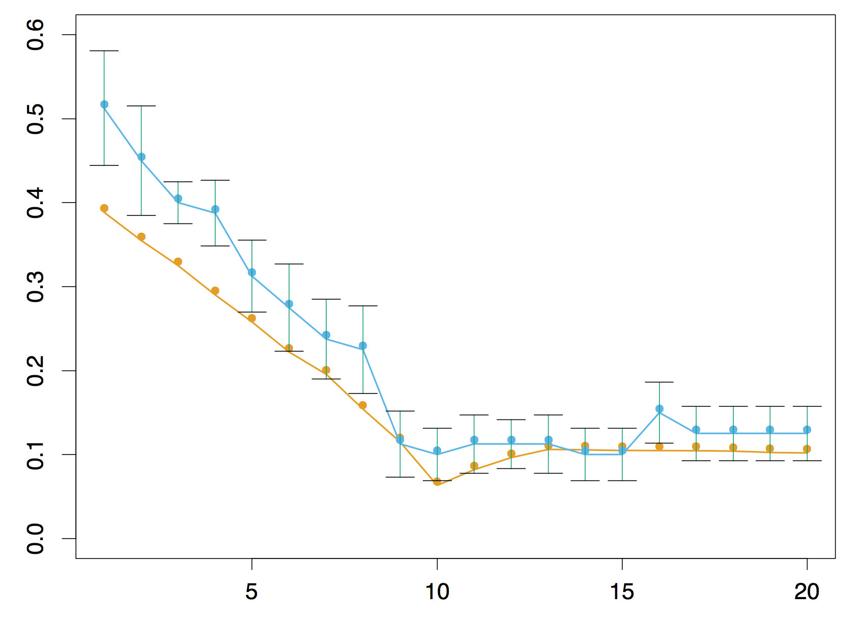
## Estimating "which is best"
vs. "performance of best"
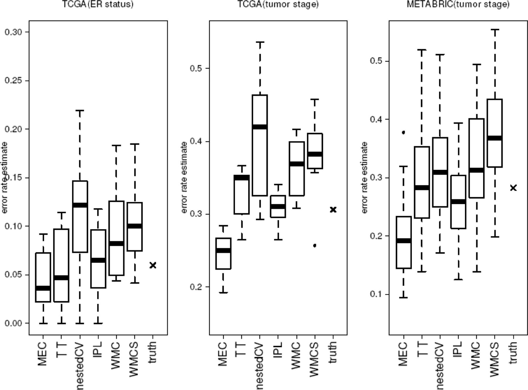
[Estimated errors using 290 model spaces.](http://bioinformatics.oxfordjournals.org/content/30/22/3152.long)
## Nested CV for Model Evaluation {.smaller}
- Divide the instances into $k$ "outer" folds of size $n/k$.
- Loop over the $k$ outer folds $i = 1 ... k$:
- Fold $i$ is for testing; all others for training.
- Divide the training instances into $k'$ "inner" folds of size $(n - n/k)/k'$.
- Loop over $m$ model spaces $1 ... m$
- Loop over the $k'$ inner folds $j = 1 ... k'$:
- Fold $j$ is for validation
- The rest are used for training
- Use average error over folds and SE to choose model space.
- Train on all inner folds.
- Test the model on outer test fold
## Nested CV for Model Evaluation
```{r echo=F,fig.height=6,fig.width=8.5}
library(cvTools)
set.seed(1)
processtestfold <- function(i) {
trange <- ((i-1)*fsize + 1):(i*fsize)
tf <- train[trange,] #Test fold
tr <- train[c(-trange),]
thefolds <- cvFolds(nrow(tr), K = folds, R = 1)
valerr <- NULL
for (deg in 1:min(dmax,nrow(tr)-1)) {
thecall <- call("lm",formula=y~poly(x,deg))
valerr[deg] <- cvTool(call=thecall,data=tr,y=tr$y,folds=thefolds)
}
dstar <- which.min(valerr)
modstar <- lm(y~poly(x,dstar),data=tr)
testerr <- mean((tf$y - predict(modstar,tf))^2)
plt <- ggplot(tr,aes(x=x,y=y)) + geom_point(color="red",size=2) + geom_point(data=tf,color="green3",size=3) +
geom_smooth(data=tr,method="lm",formula=y ~ poly(x,dstar),se=F,n=200,na.rm=F,fullrange=T) +
ggtitle(sprintf("Degree: %d, Error: %.2f",dstar,testerr))
plt$testerr <- testerr
plt
}
ptplots <- lapply(1:folds,processtestfold)
terrors <- sapply(ptplots, function(e) e$testerr)
grid.arrange(grobs=ptplots,top=textGrob(sprintf("Mean MSE: %.2f, SE: %.2f",
mean(terrors),sd(terrors)/sqrt(folds)),gp=gpar(fontsize=20)))
```
## Generalization Error for degree 3 model
```{r echo=F}
dstar <- 3
bestmod <- lm(y~poly(x,dstar),data=train)
testerr <- mean((test$y - predict(bestmod,test))^2)
ggplot(train,aes(x=x,y=y)) + geom_point(color="red",size=2) +
geom_smooth(data=train,method="lm",formula=y ~ poly(x,dstar),se=F,n=200,na.rm=F,fullrange=T) +
ggtitle(sprintf("Degree: %d, Error: %.2f on test set of size 10000",dstar,testerr))
```
Minimum-CV Estimate: 128.48, Nested CV Estimate: 149.91
## Bias-correction for the CV Procedure
[Cawley, Talbot. On Over-fitting in Model Selection and Subsequent Selection Bias in Performance Evaluation. JMLR v.11, 2010.](http://jmlr.org/papers/volume11/cawley10a/cawley10a.pdf)
[Tibshirani, Tibshirani. A bias correction for the minimum error rate in cross-validation. arXiv. 2009.](http://arxiv.org/abs/0908.2904)
[Ding et al. Bias correction for selecting the minimal-error classifier from many machine learning models. Bioinformatics 30 (22). 2014.](http://bioinformatics.oxfordjournals.org/content/30/22/3152.long)
## Summary
- The training error decreases with the degree of the polynomial
$M$, i.e. *the complexity (size) of the model space*
- Generalization error decreases at first, then starts increasing
- Set aside a *validation set* helps us find a good
model space
- We then can report unbiased error estimate, using a *test
set*, **untouched during both parameter training and
validation**
- Cross-validation is a lower-variance but possibly biased version of
this approach. It is standard.
- ***If you have lots of data, just use held-out validation and test sets.***