


Next: Interpolation and Rational Reconstruction
Up: The Euclidean Algorithm
Previous: The Euclidean Algorithm
In order to analyze Algorithms 2 and 3
we introduce the following matrices
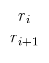
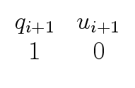
R0 =    and Qi = and Qi =  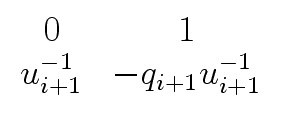  for 1 for 1  i k i k |
(12) |
with coefficients in R
mathend000#.
Then, we define
| Ri = Qi ... Q1R0 for 1 i k. |
(13) |
The following proposition collects some invariants of the
Extended Euclidean Algorithm.
Proposition 1
With the convention that
rk+1 = 0
mathend000# and
uk+1 = 1
mathend000#,
for
0  i k
mathend000# we have
i k
mathend000# we have
- (i)
mathend000#
-
Ri


 =
= 
 mathend000#,
- (ii)
mathend000#
-
Ri =


 mathend000#,
- (iii)
mathend000#
-
gcd(a, b) = gcd(ri, ri+1) = rk
mathend000#,
- (iv)
mathend000#
-
sia + tib = ri
mathend000# and
sk+1a + tk+1b = 0
mathend000#,
- (v)
mathend000#
-
siti+1 - tisi+1 = (- 1)i(u0 ... ui+1)-1
mathend000#,
- (vi)
mathend000#
-
gcd(si, ti) = 1
mathend000#,
- (vii)
mathend000#
-
gcd(ri, ti) = gcd(a, ti)
mathend000#,
- (viii)
mathend000#
- the matrices Ri
mathend000# and Qi
mathend000# are invertible;
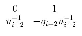
Qi-1 =

 mathend000#
and
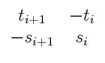
Ri-1 = (- 1)i(u0 ... ui+1)
mathend000#
and
Ri-1 = (- 1)i(u0 ... ui+1)
 mathend000#,
- (ix)
mathend000#
-
a = (- 1)i(u0 ... ui+1)(ti+1ri - tiri+1)
mathend000#,
- (x)
mathend000#
-
b = (- 1)i+1(u0 ... ui+1)(si+1ri - siri+1)
mathend000#.
Proof.
We prove (
i)
mathend000# and (ii)
mathend000# by induction on i
mathend000#.
The case i = 0
mathend000# follows immediately from the definitions
of
s0, r0, s1, r1
mathend000# and R0
mathend000#.
We assume that (i)
mathend000# and (ii)
mathend000# hold for
0 i < k
mathend000#.
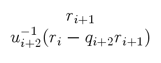
By induction hypothesis, we have
Ri+1   |
= |
Qi+1Ri |
| |
= |
Qi+1   |
| |
= |
   |
| |
= |
   |
| |
= |
   . . |
|
(14) |
Similarly, we have
| Ri+1 |
= |
Qi+1Ri |
| |
= |
Qi+1   |
| |
= |
|
| |
= |
   . . |
|
(15) |
Property (iii)
mathend000# follows from our study of Algorithm 1.
Claim (iv)
mathend000# follows (i)
mathend000# and (ii)
mathend000#.
Taking the determinant of each side of (ii)
mathend000# we prove (v)
mathend000# as follows:
| siti+1 - tisi+1 |
= |
det |
| |
= |
detRi |
| |
= |
detQi ... detQ1det |
| |
= |
(- 1)i(ui+1 ... u2)-1(u0-1u1-1 - 0). |
|
(16) |
Now, we prove (vi)
mathend000#.
If si
mathend000# and ti
mathend000# would have a non-invertible common factor, then it would
divide
siti+1 - tisi+1
mathend000#.
This contradicts (v)
mathend000# and proves (vi)
mathend000#.
We prove (vii)
mathend000#.
Let p  R
mathend000# be a divisor of ti
mathend000#.
If p | a
mathend000#, then
p | ri
mathend000# holds since we have
ri = sia + tib
mathend000#
from (i)
mathend000#.
If
p | ri
mathend000#, then
p | sia
mathend000# and, thus, p | a
mathend000# since
ti
mathend000# and si
mathend000# are relatively prime, from (vi)
mathend000#.
Therefore, (vii)
mathend000# holds.
We prove (viii)
mathend000#.
From (v)
mathend000#, we deduce that Qi
mathend000# is invertible.
Then, the invertibility of Ri
mathend000# follows easily from that of Qi
mathend000#.
It is routine to check that the proposed inverses are correct.
Finally, claims (ix)
mathend000# and (x)
mathend000# are derived from (i)
mathend000#
by multiplying each side with the inverse of Ri
mathend000# given in (viii)
mathend000#.
R
mathend000# be a divisor of ti
mathend000#.
If p | a
mathend000#, then
p | ri
mathend000# holds since we have
ri = sia + tib
mathend000#
from (i)
mathend000#.
If
p | ri
mathend000#, then
p | sia
mathend000# and, thus, p | a
mathend000# since
ti
mathend000# and si
mathend000# are relatively prime, from (vi)
mathend000#.
Therefore, (vii)
mathend000# holds.
We prove (viii)
mathend000#.
From (v)
mathend000#, we deduce that Qi
mathend000# is invertible.
Then, the invertibility of Ri
mathend000# follows easily from that of Qi
mathend000#.
It is routine to check that the proposed inverses are correct.
Finally, claims (ix)
mathend000# and (x)
mathend000# are derived from (i)
mathend000#
by multiplying each side with the inverse of Ri
mathend000# given in (viii)
mathend000#.

In the case
R =  [x]
mathend000# where
mathend000# is a field,
the following Proposition 2
shows that the degrees of
the Bézout coefficients of the
Extended Euclidean Algorithm grow linearly
whereas Proposition 3
shows that Bézout coefficients are essentially unique,
provided that their degrees are small enough.
[x]
mathend000# where
mathend000# is a field,
the following Proposition 2
shows that the degrees of
the Bézout coefficients of the
Extended Euclidean Algorithm grow linearly
whereas Proposition 3
shows that Bézout coefficients are essentially unique,
provided that their degrees are small enough.
Proof.
We only prove the first equality since the second one can be verified
in a similar way.
In fact, we prove this first equality together with
by induction on
2
i k + 1
mathend000#.
For i = 2
mathend000#, the first equality holds since we have
| degsi = deg(s0 - q2s1) = deg(1 - 0 q2) = 0 = n1 - ni-1 |
(20) |
and the inequality holds since we have
-  = degs1 < degs2 = 0. = degs1 < degs2 = 0. |
(21) |
Now we consider i  2
mathend000# and we assume that both properties
hold for
2 j i
mathend000#.
Then, by induction hypothesis, we have
2
mathend000# and we assume that both properties
hold for
2 j i
mathend000#.
Then, by induction hypothesis, we have
| degsi-1 < degsi < ni-1 - ni + degsi = degqi+1 + degsi = deg(qi+1si) |
(22) |
which implies
| degsi+1 = deg(si-1 - qi+1si) = deg(qi+1si) > degsi |
(23) |
and
degsi+1 = degqi+1 + degsi = degqi+1 + 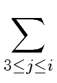 degqj = degqj = 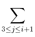 degqj degqj |
(24) |
where we used the induction hypothesis also.
Proof.
First, we observe that the index
j
mathend000# exists and is unique. Indeed,
we have
-  < degr < n
mathend000# and,
< degr < n
mathend000# and,
| - = degrk+1 < degrk < ... < degri+1 < degri < ... < dega = n. |
(28) |
Second, we claim that
holds.
Suppose that the claim is false and consider the following linear
system over R
mathend000# with


 mathend000# as unknown:
Since the matrix of this linear system is non-singular, we can solve for
f
mathend000# over the field of fractions of R
mathend000#.
Moreover, we know that
=
mathend000# is the solution.
Hence, using Cramer's rule we obtain:
a = 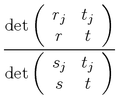 . . |
(31) |
The degree of the left hand side is n
mathend000#
while the degree of the right hand side is equal or less than:
| deg(rjt - rtj) |
|
max(degrj + degt, degr + degtj) |
| |
|
max(degr + degt, degr + n - degrj-1) |
| |
< |
max(n, degrj-1 + n - degrj-1) |
| |
= |
n, |
|
(32) |
by virtue of the definition of j
mathend000#, Relation (25) and
Proposition 2.
This leads to a contradiction.
Hence, we have
sjt = stj
mathend000#.
This implies that tj
mathend000# divides tsj
mathend000#.
Since sj
mathend000# and tj
mathend000# are relatively prime (Point (vi)
mathend000#
of Proposition 1) we deduce that
tj
mathend000# divides t
mathend000#.
So let
 [x]
mathend000# such that
we have
[x]
mathend000# such that
we have
t =  tj. tj. |
(33) |
Hence we obtain
sjtj = stj
mathend000#.
Since t  0
mathend000# holds, we have
tj 0
mathend000#, leading to
0
mathend000# holds, we have
tj 0
mathend000#, leading to
| s = sj. |
(34) |
Finally, plugging Equation (33) and Equation (34)
in Equation (25), we obtain
r = rj
mathend000#, as claimed.
Proposition 4
Let
a, b [x]
mathend000# where
mathend000# is a field.
Assume
deg(a) = n deg(b) = m
mathend000#.
- Algorithm 3 requires at most
m + 2
mathend000# inversions and
13/2m n +
 (n)
mathend000# additions
and multiplications in
mathend000#.
(n)
mathend000# additions
and multiplications in
mathend000#.
- If we do not compute the coefficients si, ti
mathend000# then
Algorithm 3 requires at most
m + 2
mathend000# inversions and
5/2m n + (n)
mathend000# additions
and multiplications in
mathend000#.
Proof.
See Theorem 3.11 in [
GG99].
Proposition 5
Let
a, b  mathend000# be multi-precision integers written with
m
mathend000# and m
mathend000# words.
Algorithm 3 can be performed in
(m n)
mathend000# word operations.
mathend000# be multi-precision integers written with
m
mathend000# and m
mathend000# words.
Algorithm 3 can be performed in
(m n)
mathend000# word operations.
Proof.
See Theorem 3.13 in [
GG99].
Next: Interpolation and Rational Reconstruction
Up: The Euclidean Algorithm
Previous: The Euclidean Algorithm
Marc Moreno Maza
2007-01-10
 degqj = n0 - ni-1
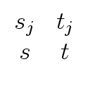

![\fbox{
\begin{minipage}{10 cm}
\begin{description}
\item[{\bf Input:}] $a,b \in ...
...\
\> {\bf return}($r_{i-2}, s_{i-2}, t_{i-2}$) \\
\end{tabbing}\end{minipage}}](img38.png)
![\fbox{
\begin{minipage}{11 cm}
\begin{description}
\item[{\bf Input:}] $a,b \in ...
...\
\> {\bf return}($r_{i-2}, s_{i-2}, t_{i-2}$) \\
\end{tabbing}\end{minipage}}](img39.png)