Let ![]()
![]()
| f = f0 + f1x + ... + fn-1xn-1 | (35) |
| f (x0) = ( ... (fn-1x0 + fn-2)x0 + ... + f1)x0 + f0 | (36) |
Li(u) =   |
(37) |
Li(uj) =  |
(38) |
Li(u) =  |
(41) |
|
(42) |
Computing f
amounting to
2 n2 - n
![]()
![]()
![]()
E :  |
(43) |
VDM(u0,..., un-1) = 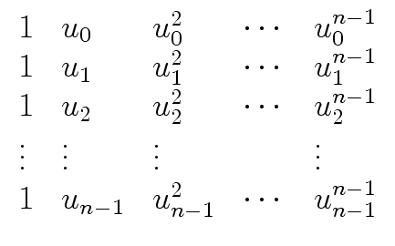 |
(44) |
 vi Li(u).
 2 i
2 i