Remark 6
Let us take a closer look at the computation of
| gi-1(2 - f gi-1) mod x2i |
(22) |
in Algorithm 2.
Consider first the product
f gi-1
mathend000#. It satisfies:
f gi-1  1 mod x2i-1 1 mod x2i-1 |
(23) |
Moreover, the polynomials f
mathend000# and gi-1
mathend000# can be seen as polynomials
with degrees less than 2i
mathend000# and 2i-1
mathend000# respectively.
Hence, there exist polynomials
S, T  R[x]
mathend000# with degree less
than 2i-1
mathend000# such that we have:
R[x]
mathend000# with degree less
than 2i-1
mathend000# such that we have:
| f gi-1 = 1 + Tx2i-1 + Sx2i. |
(24) |
We are only interested in computing T
mathend000#.
In order to avoid computing S
mathend000#, let us observe that we have
| f gi-1 (1 + S) + Tx2i-1mod x2i-1. |
(25) |
In other words, the upper part (that is, the terms of
degree at least 2i-1
mathend000#) of the convolution product of
f gi-1
mathend000# gives us exactly T
mathend000#.
So let us assume from now on that we have at hand
a primitive 2i
mathend000#-th root of unity, such that we can
compute DFT's.
Therefore, we can compute T
mathend000# at the cost of one
multiplication in degree less than 2i-1
mathend000#.
Consider now that we have computed
2 - f gi-1mod x2i
mathend000#.
Viewing
2 - f gi-1
mathend000# and gi-1
mathend000# as polynomials
with degrees less than 2i
mathend000# and 2i-1
mathend000# respectively,
there exist polynomials
U, V, W R[x]
mathend000# with degree less
than 2i-1
mathend000# such that
| gi-1(2 - f gi-1) = U + Vx2i-1 + Wx2i |
(26) |
We know that
gi-1  U mod x2i-1
mathend000#.
Hence, we are only interested in computing V
mathend000#.
Similarly to the above, we observe that
U mod x2i-1
mathend000#.
Hence, we are only interested in computing V
mathend000#.
Similarly to the above, we observe that
| gi-1(2 - f gi-1) (U + W) + Vx2i-1mod x2i-1 |
(27) |
Therefore, using DFT, we can compute V
mathend000# at the cost of one
multiplication in degree less than 2i-1
mathend000#.
It follows that, in the complexity analysis above
(in the proof of Theorem 2)
we can replace
 mathend000# by
 mathend000#
leading to
mathend000#
leading to
 mathend000#
instead of
mathend000#
instead of
 mathend000#.
 = 2gi - f gi2.
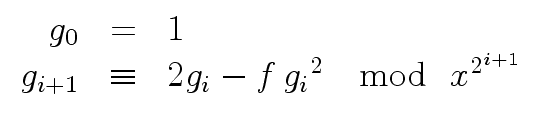


![\fbox{
\begin{minipage}{10 cm}
\begin{description}
\item[{\bf Input:}] $f \in R[...
... \mod{ \ x^{2^i}} $\ \\
\> {\bf return} $g_r$\ \\
\end{tabbing}\end{minipage}}](img35.png)