Challenges and Achievements

The main challenges of symbolic/exact computations:

• intermediate expression swell,
• complexity of symbolic computations
• implementing fast algorithms.

We iluustrate below the gap between naive and optimized implementations of the same algorithm.

Figure: Polynomial addition over $\mbox{${\mathbb Z}$}$/p$\mbox{${\mathbb Z}$}$ mathend000#.

Figure: Polynomial multiplication over $\mbox{${\mathbb Z}$}$/p$\mbox{${\mathbb Z}$}$ mathend000#.

Next, we show benchmarks between classical and FFT-based univariate polynomial multiplication.

Figure: FFT-based univariate polynomial multiplication over $\mbox{${\mathbb Z}$}$/p$\mbox{${\mathbb Z}$}$ mathend000#

Figure: Classical vs FFT-based univariate polynomial multiplication over $\mbox{${\mathbb Z}$}$/p$\mbox{${\mathbb Z}$}$ mathend000#

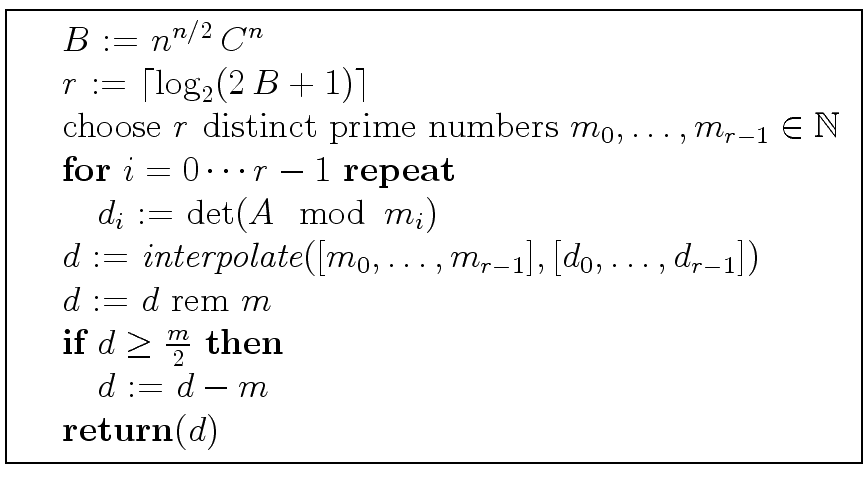
The maple work sheet Bareiss.mw iluustrates the problem of intermediate expression swell. In many situations, this problem is solved by means of modular methods. Here's an example of such method that will study in detail later

Input:

A = (a_ij) mathend000# a square matrix over $\mbox{${\mathbb Z}$}$ mathend000# of order n mathend000# with | a_ij | $\leq$ C mathend000# for 1 $\leq$ i, j $\leq$ n mathend000#.

Output:

det(A) $\in$ $\mbox{${\mathbb Z}$}$ mathend000#.

mathend000#

Another example of intermediate expression swell is given below. Consider the polynomials

$$\sp \sp \sp \sp$$ (1)

in the ring $\mbox{${\mathbb Q}$}$[x] mathend000#. The successive remainders of the Euclidean Algorithm applied to r₀ mathend000# and r₁ mathend000# are

• r₂ = x$\sp$56 + 2 x$\sp$48 + x$\sp$40 + x$\sp$10 + 1 mathend000#
• r₃ = 5 x$\sp$48 + 4 x$\sp$40 - x$\sp$34 + 2 x$\sp$26 - x$\sp$24 - 3 x$\sp$18 + 2 x$\sp$16 + 4 x$\sp$10 - 2 x$\sp$8 + 5 mathend000#
• r₄ = ${{1 \over 5} \ {x \sp {42}}}$ + ${{1 \over {25}} \ {x \sp {40}}}$ - ${{4 \over {25}} \ {x \sp {34}}}$ + ${{1 \over 5} \ {x \sp {32}}}$ + ${{3 \over {25}} \ {x \sp {26}}}$ - ${{4 \over {25}} \ {x \sp {24}}}$ - ${{2 \over {25}} \ {x \sp {18}}}$ - ${{2 \over {25}} \ {x \sp {16}}}$ + ${{1 \over {25}} \ {x \sp {10}}}$ - ${{{13} \over {25}} \ {x \sp 8}}$ - ${1 \over 5}$ mathend000#
• r₅ = ${{{1001} \over {625}} \ {x \sp {40}}}$ - ${{{29} \over {25}} \ {x \sp {38}}}$ + ${{{29} \over {125}} \ {x \sp {36}}}$ - ${{{154} \over {625}} \ {x \sp {34}}}$ - ${{{74} \over {125}} \ {x \sp {32}}}$ + ${{{23} \over {25}} \ {x \sp {30}}}$ - ${{{23} \over {125}} \ {x \sp {28}}}$ + ${{{273} \over {625}} \ {x \sp {26}}}$ + ${{{121} \over {625}} \ {x \sp {24}}}$ + ${{8 \over {25}} \ {x \sp {22}}}$ - ${{8 \over {125}} \ {x \sp {20}}}$ - ${{{367} \over {625}} \ {x \sp {18}}}$ + ${{{123} \over {625}} \ {x \sp {16}}}$ + ${{{66} \over {25}} \ {x \sp {14}}}$ - ${{{66} \over {125}} \ {x \sp {12}}}$ + ${{{566} \over {625}} \ {x \sp {10}}}$ - ${{{263} \over {625}} \ {x \sp 8}}$ + x$\sp$6 - ${{1 \over 5} \ {x \sp 4}}$ + ${{1 \over {25}} \ {x \sp 2}}$ + ${{124} \over {125}}$ mathend000#
• r₆ = ${{{525625} \over {1002001}} \ {x \sp {38}}}$ + ${{{20000} \over {1002001}} \ {x \sp {36}}}$ - ${{{3750} \over {13013}} \ {x \sp {34}}}$ + ${{{768750} \over {1002001}} \ {x \sp {32}}}$ - ${{{416875} \over {1002001}} \ {x \sp {30}}}$ - ${{{166875} \over {1002001}} \ {x \sp {28}}}$ + ${{{2500} \over {11011}} \ {x \sp {26}}}$ - ${{{101250} \over {91091}} \ {x \sp {24}}}$ - ${{{145000} \over {1002001}} \ {x \sp {22}}}$ + ${{{404375} \over {1002001}} \ {x \sp {20}}}$ - ${{{184375} \over {1002001}} \ {x \sp {18}}}$ - ${{{2166250} \over {1002001}} \ {x \sp {16}}}$ - ${{{108750} \over {91091}} \ {x \sp {14}}}$ - ${{{23750} \over {91091}} \ {x \sp {12}}}$ - ${{{60000} \over {1002001}} \ {x \sp {10}}}$ - ${{{2987500} \over {1002001}} \ {x \sp 8}}$ - ${{{453125} \over {1002001}} \ {x \sp 6}}$ + ${{{90625} \over {1002001}} \ {x \sp 4}}$ - ${{{643750} \over {1002001}} \ {x \sp 2}}$ - ${{1575625} \over {1002001}}$ mathend000#
• r₇ = ${{{511511} \over {707281}} \ {x \sp {36}}}$ - ${{{1439438} \over {707281}} \ {x \sp {34}}}$ + ${{{1088087} \over {707281}} \ {x \sp {32}}}$ + ${{{7007} \over {24389}} \ {x \sp {30}}}$ - ${{{558558} \over {707281}} \ {x \sp {28}}}$ + ${{{1924923} \over {707281}} \ {x \sp {26}}}$ - ${{{861861} \over {707281}} \ {x \sp {24}}}$ - ${{{19019} \over {24389}} \ {x \sp {22}}}$ + ${{{634634} \over {707281}} \ {x \sp {20}}}$ + ${{{2466464} \over {707281}} \ {x \sp {18}}}$ - ${{{525525} \over {707281}} \ {x \sp {16}}}$ + ${{{10010} \over {24389}} \ {x \sp {14}}}$ - ${{{420420} \over {707281}} \ {x \sp {12}}}$ + ${{{4358354} \over {707281}} \ {x \sp {10}}}$ - ${{{2640638} \over {707281}} \ {x \sp 8}}$ - ${{{5005} \over {24389}} \ {x \sp 6}}$ + ${{{30030} \over {24389}} \ {x \sp 4}}$ + ${{{1477476} \over {707281}} \ {x \sp 2}}$ - ${{1178177} \over {707281}}$ mathend000#
• r₈ = ${{{1396901} \over {261121}} \ {x \sp {34}}}$ - ${{{1306073} \over {261121}} \ {x \sp {32}}}$ - ${{{31117} \over {37303}} \ {x \sp {30}}}$ - ${{{252300} \over {261121}} \ {x \sp {28}}}$ - ${{{2249675} \over {261121}} \ {x \sp {26}}}$ + ${{{140447} \over {37303}} \ {x \sp {24}}}$ + ${{{407044} \over {261121}} \ {x \sp {22}}}$ - ${{{1982237} \over {261121}} \ {x \sp {20}}}$ - ${{{487780} \over {37303}} \ {x \sp {18}}}$ - ${{{65598} \over {37303}} \ {x \sp {16}}}$ - ${{{802314} \over {261121}} \ {x \sp {14}}}$ - ${{{248936} \over {37303}} \ {x \sp {12}}}$ - ${{{102602} \over {5329}} \ {x \sp {10}}}$ + ${{{2434695} \over {261121}} \ {x \sp 8}}$ - ${{{458345} \over {261121}} \ {x \sp 6}}$ - ${{{1977191} \over {261121}} \ {x \sp 4}}$ - ${{{1869543} \over {261121}} \ {x \sp 2}}$ + ${{932669} \over {261121}}$ mathend000#
• r₉ = ${{{1451751} \over {2758921}} \ {x \sp {32}}}$ + ${{{785918} \over {2758921}} \ {x \sp {30}}}$ + ${{{494137} \over {2758921}} \ {x \sp {28}}}$ + ${{{91469} \over {2758921}} \ {x \sp {26}}}$ - ${{{1803830} \over {2758921}} \ {x \sp {24}}}$ + ${{{222796} \over {250811}} \ {x \sp {22}}}$ + ${{{2809989} \over {2758921}} \ {x \sp {20}}}$ + ${{{1538110} \over {2758921}} \ {x \sp {18}}}$ - ${{{2954091} \over {2758921}} \ {x \sp {16}}}$ + ${{{2029692} \over {2758921}} \ {x \sp {14}}}$ + ${{{1194718} \over {2758921}} \ {x \sp {12}}}$ + ${{{40369} \over {2758921}} \ {x \sp {10}}}$ - ${{{4301598} \over {2758921}} \ {x \sp 8}}$ + ${{{1421091} \over {2758921}} \ {x \sp 6}}$ + ${{{1051638} \over {2758921}} \ {x \sp 4}}$ - ${{{811468} \over {2758921}} \ {x \sp 2}}$ - ${{2893282} \over {2758921}}$ mathend000#
• r₁₀ = ${{{2444992} \over {8071281}} \ {x \sp {30}}}$ + ${{{2089538} \over {8071281}} \ {x \sp {28}}}$ - ${{{2219096} \over {8071281}} \ {x \sp {26}}}$ - ${{{22750717} \over {8071281}} \ {x \sp {24}}}$ + ${{{6844981} \over {8071281}} \ {x \sp {22}}}$ + ${{{1019854} \over {2690427}} \ {x \sp {20}}}$ + ${{{9319871} \over {8071281}} \ {x \sp {18}}}$ - ${{{12728243} \over {2690427}} \ {x \sp {16}}}$ + ${{{597960} \over {896809}} \ {x \sp {14}}}$ - ${{{486673} \over {8071281}} \ {x \sp {12}}}$ - ${{{4801951} \over {8071281}} \ {x \sp {10}}}$ - ${{{9713528} \over {2690427}} \ {x \sp 8}}$ + ${{{352132} \over {896809}} \ {x \sp 6}}$ + ${{{191015} \over {896809}} \ {x \sp 4}}$ - ${{{1376969} \over {8071281}} \ {x \sp 2}}$ - ${{18359033} \over {8071281}}$ mathend000#
• r₁₁ = ${{{821049} \over {541696}} \ {x \sp {28}}}$ + ${{{1230153} \over {135424}} \ {x \sp {26}}}$ - ${{{7537173} \over {1083392}} \ {x \sp {24}}}$ + ${{{1423341} \over {1083392}} \ {x \sp {22}}}$ - ${{{804003} \over {541696}} \ {x \sp {20}}}$ + ${{{19361415} \over {1083392}} \ {x \sp {18}}}$ - ${{{9889521} \over {1083392}} \ {x \sp {16}}}$ + ${{{309669} \over {135424}} \ {x \sp {14}}}$ + ${{{2951799} \over {1083392}} \ {x \sp {12}}}$ + ${{{12275961} \over {1083392}} \ {x \sp {10}}}$ - ${{{1082421} \over {135424}} \ {x \sp 8}}$ + ${{{184665} \over {270848}} \ {x \sp 6}}$ + ${{{71025} \over {47104}} \ {x \sp 4}}$ + ${{{7338303} \over {1083392}} \ {x \sp 2}}$ - ${{4707537} \over {1083392}}$ mathend000#
• r₁₂ = ${{{2879600} \over {83521}} \ {x \sp {26}}}$ - ${{{2819432} \over {83521}} \ {x \sp {24}}}$ + ${{{687608} \over {83521}} \ {x \sp {22}}}$ - ${{{1300512} \over {83521}} \ {x \sp {20}}}$ + ${{{5881560} \over {83521}} \ {x \sp {18}}}$ - ${{{4015064} \over {83521}} \ {x \sp {16}}}$ + ${{{681168} \over {83521}} \ {x \sp {14}}}$ + ${{{130456} \over {83521}} \ {x \sp {12}}}$ + ${{{3484776} \over {83521}} \ {x \sp {10}}}$ - ${{{3296176} \over {83521}} \ {x \sp 8}}$ + ${{{218224} \over {83521}} \ {x \sp 6}}$ + ${{{112424} \over {83521}} \ {x \sp 4}}$ + ${{{2110296} \over {83521}} \ {x \sp 2}}$ - ${{1857480} \over {83521}}$ mathend000#
• r₁₃ = ${{{489294629} \over {244922500}} \ {x \sp {24}}}$ - ${{{84853001} \over {244922500}} \ {x \sp {22}}}$ + ${{{15566407} \over {122461250}} \ {x \sp {20}}}$ - ${{{51711059} \over {48984500}} \ {x \sp {18}}}$ + ${{{848011833} \over {244922500}} \ {x \sp {16}}}$ - ${{{11383999} \over {61230625}} \ {x \sp {14}}}$ + ${{{66509593} \over {244922500}} \ {x \sp {12}}}$ + ${{{44817253} \over {244922500}} \ {x \sp {10}}}$ + ${{{322278061} \over {122461250}} \ {x \sp 8}}$ - ${{{7199857} \over {61230625}} \ {x \sp 6}}$ - ${{{2507653} \over {244922500}} \ {x \sp 4}}$ + ${{{1074213} \over {244922500}} \ {x \sp 2}}$ + ${{79874687} \over {48984500}}$ mathend000#
• r₁₄ = ${{{101577545700} \over {2866455549721}} \ {x \sp {22}}}$ + ${{{367076384000} \over {2866455549721}} \ {x \sp {20}}}$ - ${{{333608859000} \over {2866455549721}} \ {x \sp {18}}}$ + ${{{272633704600} \over {2866455549721}} \ {x \sp {16}}}$ + ${{{73493401600} \over {2866455549721}} \ {x \sp {14}}}$ + ${{{181230098700} \over {2866455549721}} \ {x \sp {12}}}$ - ${{{95624598700} \over {2866455549721}} \ {x \sp {10}}}$ - ${{{70116632400} \over {2866455549721}} \ {x \sp 8}}$ + ${{{95985644200} \over {2866455549721}} \ {x \sp 6}}$ + ${{{93781623400} \over {2866455549721}} \ {x \sp 4}}$ - ${{{233932944800} \over {2866455549721}} \ {x \sp 2}}$ + ${{36036190800} \over {2866455549721}}$ mathend000#
• r₁₅ = ${{{179398565293636} \over {10531900693521}} \ {x \sp {20}}}$ - ${{{54943352709941} \over {3510633564507}} \ {x \sp {18}}}$ + ${{{117687363770051} \over {10531900693521}} \ {x \sp {16}}}$ + ${{{9087736866857} \over {10531900693521}} \ {x \sp {14}}}$ + ${{{27503113958149} \over {3510633564507}} \ {x \sp {12}}}$ - ${{{29314013696810} \over {10531900693521}} \ {x \sp {10}}}$ - ${{{7870248236452} \over {3510633564507}} \ {x \sp 8}}$ + ${{{27346896912740} \over {10531900693521}} \ {x \sp 6}}$ + ${{{61025918153225} \over {10531900693521}} \ {x \sp 4}}$ - ${{{95570962105003} \over {10531900693521}} \ {x \sp 2}}$ + ${{2527399767739} \over {1170211188169}}$ mathend000#
• r₁₆ = ${{{2517066778702173} \over {11227749627077776}} \ {x \sp {18}}}$ - ${{{3818112212630217} \over {11227749627077776}} \ {x \sp {16}}}$ + ${{{381679883443605} \over {11227749627077776}} \ {x \sp {14}}}$ - ${{{1538892758851425} \over {11227749627077776}} \ {x \sp {12}}}$ - ${{{388249516683645} \over {5613874813538888}} \ {x \sp {10}}}$ - ${{{691018345032231} \over {2806937406769444}} \ {x \sp 8}}$ - ${{{60451575413454} \over {701734351692361}} \ {x \sp 6}}$ - ${{{963937271272515} \over {11227749627077776}} \ {x \sp 4}}$ - ${{{170313672155631} \over {11227749627077776}} \ {x \sp 2}}$ - ${{2469351761856789} \over {11227749627077776}}$ mathend000#
• r₁₇ = ${{{849182055193466800} \over {601565221018811449}} \ {x \sp {16}}}$ + ${{{343702214828429548} \over {601565221018811449}} \ {x \sp {14}}}$ + ${{{682224379091263268} \over {601565221018811449}} \ {x \sp {12}}}$ + ${{{673295990111439292} \over {601565221018811449}} \ {x \sp {10}}}$ + ${{{547091169006122260} \over {601565221018811449}} \ {x \sp 8}}$ + ${{{460333296636481632} \over {601565221018811449}} \ {x \sp 6}}$ + ${{{383125215937085648} \over {601565221018811449}} \ {x \sp 4}}$ + ${{{294034834904863988} \over {601565221018811449}} \ {x \sp 2}}$ + ${{429248529314696936} \over {601565221018811449}}$ mathend000#
• r₁₈ = ${{{8093646079436159529} \over {64225707449292490000}} \ {x \sp {14}}}$ + ${{{8963514770014081139} \over {64225707449292490000}} \ {x \sp {12}}}$ + ${{{36664367930801793141} \over {64225707449292490000}} \ {x \sp {10}}}$ - ${{{5166279318582404449} \over {12845141489858498000}} \ {x \sp 8}}$ + ${{{1655921845497232367} \over {8028213431161561250}} \ {x \sp 6}}$ + ${{{553008257063777544} \over {4014106715580780625}} \ {x \sp 4}}$ + ${{{5923554723478841499} \over {64225707449292490000}} \ {x \sp 2}}$ - ${{311063035823698661} \over {32112853724646245000}}$ mathend000#
• r₁₉ = - ${{{321061300213427783600} \over {108894438325788541209}} \ {x \sp {12}}}$ + ${{{260178685392579511400} \over {36298146108596180403}} \ {x \sp {10}}}$ - ${{{50329696078066373200} \over {15556348332255505887}} \ {x \sp 8}}$ + ${{{65235764858211154700} \over {108894438325788541209}} \ {x \sp 6}}$ + ${{{17696479989822163900} \over {36298146108596180403}} \ {x \sp 4}}$ + ${{{34027149119020814900} \over {36298146108596180403}} \ {x \sp 2}}$ + ${{49162422013935572500} \over {108894438325788541209}}$ mathend000#
• r₂₀ = ${{{4829115100553781731631} \over {401242596572878762276}} \ {x \sp {10}}}$ - ${{{2757078265767537479145} \over {401242596572878762276}} \ {x \sp 8}}$ + ${{{2023158681969000162489} \over {802485193145757524552}} \ {x \sp 6}}$ + ${{{1601998453967540114703} \over {802485193145757524552}} \ {x \sp 4}}$ + ${{{1613072222486808321189} \over {802485193145757524552}} \ {x \sp 2}}$ + ${{373138984504746247389} \over {802485193145757524552}}$ mathend000#
• r₂₁ = - ${{{37302462364041459452987} \over {214155589697125984393929}} \ {x \sp 8}}$ + ${{{2941869220852112384353} \over {142770393131417322929286}} \ {x \sp 6}}$ - ${{{10204521350404552579523} \over {428311179394251968787858}} \ {x \sp 4}}$ - ${{{19661683201604262591215} \over {428311179394251968787858}} \ {x \sp 2}}$ - ${{34803628802314892079373} \over {428311179394251968787858}}$ mathend000#
• r₂₂ = ${{{1062516113981431489446399} \over {55486579353465726911265604}} \ {x \sp 6}}$ - ${{{1984430997558975837247707} \over {55486579353465726911265604}} \ {x \sp 4}}$ - ${{{9998817850051608518344935} \over {55486579353465726911265604}} \ {x \sp 2}}$ + ${{13859935515210895384665945} \over {55486579353465726911265604}}$ mathend000#
• r₂₃ = ${{{67553029541578289076276832} \over {5271590127845040063150969}} \ {x \sp 4}}$ + ${{{6469282280812842012581780} \over {1757196709281680021050323}} \ {x \sp 2}}$ - ${{117836407258993771969728352} \over {5271590127845040063150969}}$ mathend000#
• r₂₄ = - ${{{144893287293662194035293991} \over {20560880907683469568857664}} \ {x \sp 2}}$ + ${{23864545606303620039559371} \over {2570110113460433696107208}}$ mathend000#
• r₂₅ = ${{1474954192646018616432640872} \over {3982491846600722083699067449}}$ mathend000#
• r₂₆ = 0 mathend000#

We will study modular methods for the Euclidean Algorithm too.