Next: The Chinese Remaindering Algorithm Up: Interpolation and Rational Reconstruction Previous: Interpolation and Rational Reconstruction
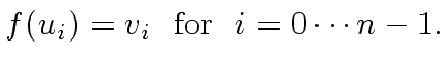
Let ![]() be a field and let
be a field and let
 be a sequence of pairwise distinct elements of
 ![]() .
.
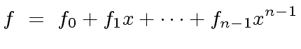
![$ {\bf k}[x]$](img191.png) with degree
with degree  , say
, say
 |
(35) |
 using Horner's rule
 |
(36) |
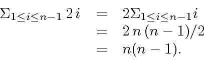
additions and
multiplications leading to
 operations in the base field
  .
.
 the
the 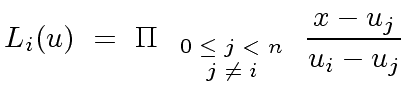 |
(37) |
 |
(38) |
 be in
be in ![$ f \in {\bf k}[x]$](img202.png) with degree less than
with degree less than
of degree less than  or computing an interpolating polynomial at these points
can be done in
or computing an interpolating polynomial at these points
can be done in
 operations in
at one point costs
operations in
amounts to
operations in
at one point costs
operations in
amounts to
 .
Let us prove now that interpolating a polynomial at
can be done in
operations in
.
Let us prove now that interpolating a polynomial at
can be done in
operations in  .
Consider
.
Consider  ,
,
 , ...
, ...
 where
where  .
Let
.
Let
 and
and
 for
for
 |
(41) |
's let us start with that of
of degree
of degree  plus
(of degree
plus
(of degree  (of degree
  but without constant term)
 amounts to
 |
(42) |
 steps, each step requiring
computing each
steps, each step requiring
computing each  's
amounts to
operations in the base field
's amounts to
.
Then computing each
's
amounts to
operations in the base field
's amounts to
.
Then computing each
 from the
's costs
's from scratch
amounts to
from the
's costs
's from scratch
amounts to
 .
.
Computing ![]() from the
's requires
from the
's requires
(which is a polynomial of degree
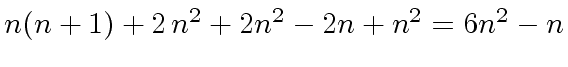
) by the number  leading to
additions
of polynomials of degree at most
costing
leading to
additions
of polynomials of degree at most
costing  operations in
  .
Finally the total cost is
.
Finally the total cost is
 .
.
 |
(43) |
.
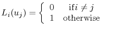
It is obvious that  |
(44) |
 for all
 .
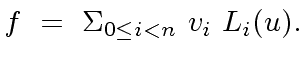
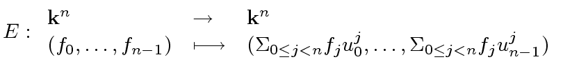
To conclude observe that both
evaluation and interpolation
are linear maps between coefficients and value vectors.
.
To conclude observe that both
evaluation and interpolation
are linear maps between coefficients and value vectors.