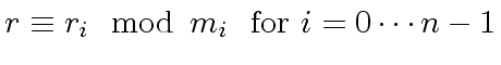
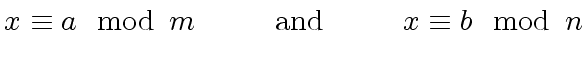
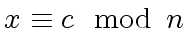
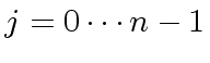
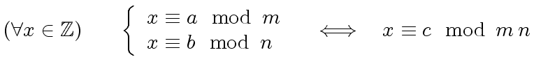
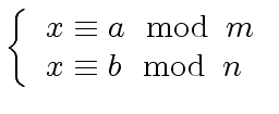
We start with the elementary case of the
Chinese Remaindering Theorem
(Theorem 1).
Then we give a much more abstract version
(Theorem 2).
Then we state the Chinese Remaindering Theorem
and
the
Chinese Remaindering Algorithm
in the context of Euclidean domains.
Proof.
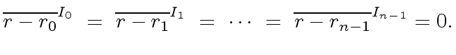
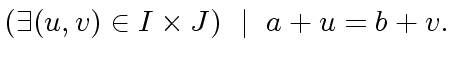
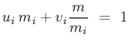
First observe that Relation (
46) implies
 |
(48) |
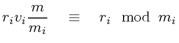
Now assume that
holds.
This implies
 |
(49) |
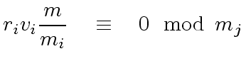
Thus Relations (
48) and (
49) lead to
 |
(50) |
Conversly
-
 implies
 that is
  divides
  and
and
-
 implies
 that is
  divides
.
divides
.
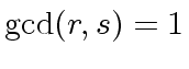
Since
and
are relatively prime it follows that

divides
.
(Gauss Lemma).

Proof.
The first statement is obvious.
Let us prove the second one.
Let
be in

.
We look for the pre-image of
.
Hence we look for

such that
 |
(53) |
that is
 |
(54) |
or
 |
(55) |
At this point of the proof we need the following lemma.
Proof.
The equation
means that the residue classe of

in

is equal
to the residue classe of

in

.
More formally we have
 |
(57) |
or equivalently
 |
(58) |
Since these sets are non empty this implies
 |
(59) |
Since

is an ideal we have
and thus
 |
(60) |
The lemma is proved.
CONTINUING THEOREM'S
Proof.
With the previous lemma
Relation (
55),
for all

such that
holds, leads to
 |
(61) |
or equivalently
 |
(62) |
Relation (
62) is a necessary condition
for the existence of a pre-image of
via the homomorphism

.
Therefore we proved the second statement of the theorem.
Let us prove the third one.
Let us ssume first that
is surjective.
Let
be such that
.
There exists  such that
 |
(63) |
Hence
 |
(64) |
which implies
.
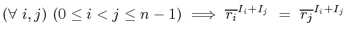
Conversly, let us assume that the ideals
are pairwise coprime.
Let

be in the range
and consider
the product

of all ideals
except

.
It is a classical result that
and
are coprime.
Let

and

such that
.
Observe that for all
we have
 |
(65) |
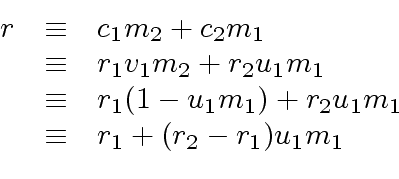
Now consider
.
Then
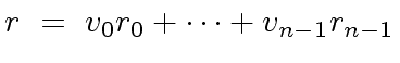 |
(66) |
satisfies
|
(67) |
This concludes the proof of the theorem.
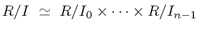
Proof.
The following ring isomorphism follows from Theorem
2
 |
(70) |
It is a well known fact that if the ideals
are pairwise coprime
(
for every
with
)
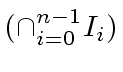
then their product is equal to their intersection [
van91].
Therefore, we have the ring isomorphism of the statement.
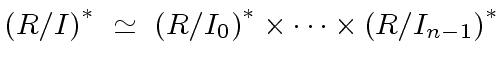
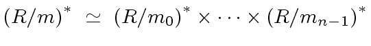
The group isomorphism follows from the previous ring isomorphism
and the fact that the element
 |
(71) |
is a unit iff every

is a unit of

.
From now on
denotes an Euclidean domain.
Proof.
Assume that the algorithm terminates without error,
that is the case if every

is
the gcd of

and

(which are assumed to be coprime).
Then, for
we have
 |
(74) |
Hence
 |
(75) |
and for
with

we have
 |
(76) |
The specification of Algorithm
4 follow
easily from Relation (
75) and (
76).
Proof.
Except for the complexity result (that can be found
in [
GG99] as Theorem 5.7) and the uniqueness, this theorem follows
from Algorithm
4.
The uniqueness follows from the constraint
.
Indeed, assume that there are two polynomials

and

solutions
of (
80).
Then we have
 |
(81) |
and thus
 |
(82) |
Hence
divides

although
holds.
Therefore

.
Proof.
Except for the complexity result (that can be found
in [
GG99] as Theorem 5.8) and the uniqueness,
this theorem follows
from Algorithm
4.
The proof of the uniqueness is quite easy to establish.
We reproduce below the ALDOR code for the Chinese Remaindering Algorithm.
More precisely, the operation interpolate satisfies exactly the
specification of Algorithm 4.
After the definition of the ChineseRemaindering domain
we prove that its operation combine satisifies the
specification of Algorithm 4
for the case of two moduli  and
and  .
The reader is left with the proof of the operation interpolate
which implements the general case (with
.
The reader is left with the proof of the operation interpolate
which implements the general case (with  moduli).
ChineseRemaindering(E: EuclideanDomain): with {
combine: (E, E) -> (E, E) -> E;
interpolate: (List E, List E) -> E;
} == add {
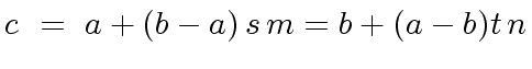
combine(m1: E, m2: E): (E, E) -> E == {
local u1: E;
assert(m1 = unitCanonical m1);
assert(m2 = unitCanonical m2);
fn(r1: E, r2: E): E == {
r1__new := r1 rem m1;
r := (r2 - r1__new) rem m2 ;
r := (r * u1) rem m2 ;
r := r1__new + r * m1;
}
(u1, u2, g) := extendedEuclidean(m1, m2);
fn
}
interpolate(lm: List E, lr: List E): E == {
m := first lm;
r := first lr rem m;
for mi in rest lm for ri in rest lr repeat {
r := combine(m, mi)(r, ri);
m := m * mi;
}
return r;
}
}
Marc Moreno Maza
2008-01-07
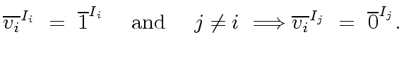
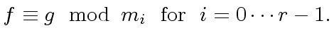
 be such that
 .
For every
.
For every
 there exists
 such that
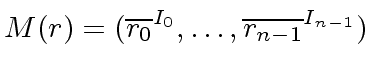
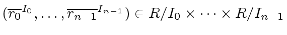
 be ideals of
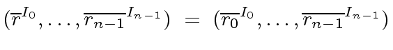
  (additions and multiplications are computed componentwise)
together with the homomorphism
(additions and multiplications are computed componentwise)
together with the homomorphism
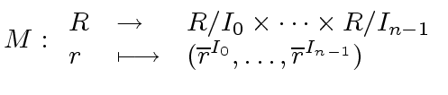
 .
.
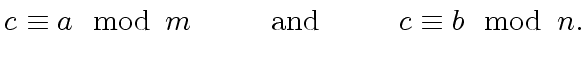
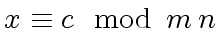
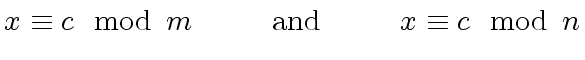
 be two elements of the ring
  be two ideals of
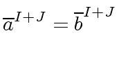
 be
be  we have
 .)
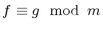
Let
.)
Let
 .
Then, we have the ring isomorphism
.
Then, we have the ring isomorphism
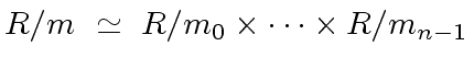
 .
.
 ,
...
,
...
 .
.
 .
This follows from the fact the
.
This follows from the fact the 
![$ R = {\bf k}[x]$](img19.png) for a field
for a field  be polynomials
pairwise coprime (
be polynomials
pairwise coprime (
 ).
Let
).
Let  let
let
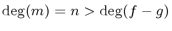
 be the degree of
  be the degree of
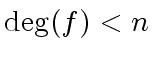
 ![$ f_i \in {\bf k}[x]$](img336.png) be a polynomial with degree
be a polynomial with degree
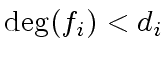 .
Then there is a unique polynomial
.
Then there is a unique polynomial
![$ f \in {\bf k}[x]$](img202.png) such that
such that
 operations in
  be in
be in
 be such that
 for
for
 .
Then there is a unique
.
Then there is a unique  such that

 .
.
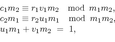
 := extendedEuclidean(
 rem
rem 
 := extendedEuclidean(
 )
)
 rem
rem 
 rem
rem 
![\fbox{
\begin{minipage}{12 cm}
\begin{description}
\item[{\bf Input:}] $m_0, \do...
...= $r + c_i \frac{m}{m_i}$\ \\
\> {\bf return} $r$
\end{tabbing}\end{minipage}}](img318.png)