Next: Division with remainder using Newton Up: Division with remainder using Newton Previous: The quotient as a modular
![$ f \in R[x]$](img55.png) and
and
 such that
  compute the polynomials
![$ g \in R[x]$](img58.png) such that
such that
 is a multiple of
then
is a multiple of
then
 must be 0
.
Hence there is a constant
must be 0
.
Hence there is a constant  and polynomials
  with degree less than
 such that
 |
(9) |
 is a multiple of
 .
Then by induction on
.
Then by induction on  .
.
![$ R[x]/\langle x^{\ell} \rangle$](img74.png) ,
a solution of this equation can be viewed as
an approximation of a more general problem.
Think of truncated Taylor expansions!
So let us recall from numerical analysis the celebrated Newton iteration
and let
,
a solution of this equation can be viewed as
an approximation of a more general problem.
Think of truncated Taylor expansions!
So let us recall from numerical analysis the celebrated Newton iteration
and let
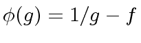
 be an equation that we want to solve,
where
be an equation that we want to solve,
where
 is a differentiable function.
From a suitable initial approximation
is a differentiable function.
From a suitable initial approximation 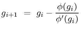 |
(10) |
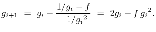
 and the Newton iteration step is
 |
(11) |
![$ R[x]$](img5.png) such that
.
Let
such that
.
Let
 be the sequence of polynomials defined
for all
be the sequence of polynomials defined
for all  by
by
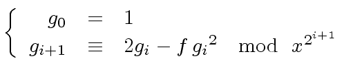 |
(12) |
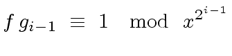
we have
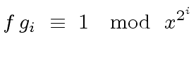 |
(13) |
.
For 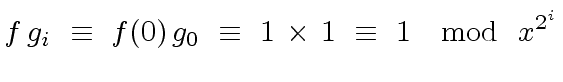 |
(14) |
 |
(15) |
 means that
 .
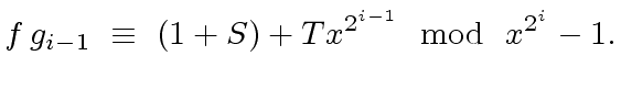
Thus
.
Thus
 .
.
 , any pair of polynomials in
of degree less than
, any pair of polynomials in
of degree less than  operations of
  , for every
 ,
with
,
with  . This implies the superlinearity
properties, that is, for every
. This implies the superlinearity
properties, that is, for every
 for some
  operations in
  .
.
 |
(17) |
 |
(18) |
 etc.
etc.
 |
(19) |
 operations in
The cost for the ![]() -th iteration is
-th iteration is
 for the computation of
 ,
,
 for the product
 ,
,
 modulo
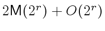
 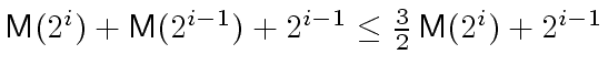 , resulting in a total running time:
 for all

|
(21) |
 .
.
 is a unit different from
instead of
is not a unit, then no inverse of
is a unit different from
instead of
is not a unit, then no inverse of  implies
 which says that
is a unit.
which says that
is a unit.
 |
(22) |
 . It satisfies:
 |
(23) |
can be seen as polynomials
with degrees less than ![$ S, T \in R[x]$](img146.png) with degree less
than
with degree less
than 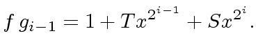 |
(24) |
 |
(25) |
gives us exactly
So let us assume from now on that we have at hand
a primitive ![]() -th root of unity, such that we can
compute DFT's.
Therefore, we can compute
-th root of unity, such that we can
compute DFT's.
Therefore, we can compute ![]() at the cost of one
multiplication in degree less than
at the cost of one
multiplication in degree less than ![]() .
.
Consider now that we have computed
 .
Viewing
.
Viewing
 and
as polynomials
with degrees less than
and
as polynomials
with degrees less than ![]() and
and ![]() respectively,
there exist polynomials
respectively,
there exist polynomials
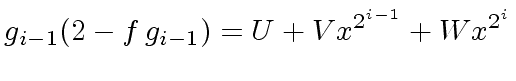
![$ U, V, W \in R[x]$](img154.png) with degree less
than
with degree less
than ![]() such that
such that
 |
(26) |
 .
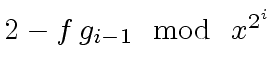
Hence, we are only interested in computing
.
Hence, we are only interested in computing 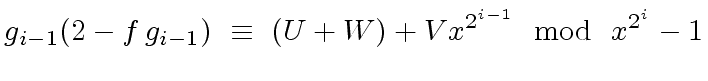 |
(27) |
It follows that, in the complexity analysis above
(in the proof of Theorem 2)
we can replace
 by
by
 leading to
 instead of
 .
.
![\fbox{
\begin{minipage}{10 cm}
\begin{description}
\item[{\bf Input:}] $f \in R[...
... \mod{ \ x^{2^i}} $\ \\
\> {\bf return} $g_r$\ \\
\end{tabbing}\end{minipage}}](img95.png)