


Next: Modular computation of the determinant
Up: Modular Algorithms and interpolation
Previous: Evaluation, interpolation
We start with the elementary case of the
Chinese Remaindering Theorem
(Theorem 2).
Then we give a much more abstract version
(Theorem 3).
Then we state the Chinese Remaindering Theorem
and
the
Chinese Remaindering Algorithm
in the context of Euclidean domains.
Theorem 2 (Sun-Tsu, first century AD)
Let
m and
n be two relatively prime integers.
Let
s,
t 

be such that
s m +
t n = 1.
For every
a,
b there exists
c
such that
where a convenient
c is given by
| c = a + (b - a) s m = b + (a - b)t n |
(37) |
Therefore for every
a,
b the system
of equations
 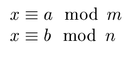 |
(38) |
has a solution.
Proof.
First observe that Relation (
37) implies
c  a mod m and c b mod n. a mod m and c b mod n. |
(39) |
Now assume that
x  c
c mod
m n holds.
This implies
| x c mod m and x c mod n |
(40) |
Thus Relations (
39) and (
40) lead to
| x a mod m and x b mod n |
(41) |
Conversly
-
x a mod m implies
x c mod m that is m divides x - c and
-
x b mod n implies
x c mod n that is n divides x - c.
Since
m and
n are relatively prime it follows that
m n divides
x -
c.
(Gauss Lemma).

Theorem 3
Let
R be a commutative ring with unity and
I0,
I1,...,
In-1 be ideals of
R.
We consider the direct product of residue class rings
R/
I0×
... ×
R/
In-1
(additions and multiplications are computed componentwise)
together with the homomorphism
M : 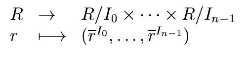 |
(42) |
Then we have
Proof.
The first statement is obvious.
Let us prove the second one.
Let
r,
r0,
r1,...,
rn-1 be in
R.
We look for the pre-image of
(

,...,
).
Hence we look for
r such that
M(r) = ( ,..., ,..., ) ) |
(44) |
that is
or
At this point of the proof we need the following lemma.
Lemma 1
Let
a,
b be two elements of the ring
R (again commutative
and with unity).
Let
I,
J be two ideals of
R such that

=

.
Then we have
 = =  |
(47) |
Proof.
The equation
=
means that the residue classe of
a in
R/
I is equal
to the residue classe of
b in
R/
J.
More formally we have
{x  R | a - x I} = {x R | b - x J} R | a - x I} = {x R | b - x J} |
(48) |
or equivalently
{x R | ( u I) | x = a + u} = {x R | (v I) | x = b + v} u I) | x = a + u} = {x R | (v I) | x = b + v} |
(49) |
Since these sets are non empty this implies
| ((u, v) I×J) | a + u = b + v. |
(50) |
Since
J is an ideal we have -
v J and thus
| a - b I + J |
(51) |
The lemma is proved.
CONTINUING THEOREM'S
Proof.
With the previous lemma
Relation
46 leads to
 = =  |
(52) |
for
i,
j such that
0
 i
i <
j n - 1 or equivalently
 = =  |
(53) |
Relation (
53) is a necessary condition
for the existence of a pre-image of
r via the homomorphism
M.
Therefore we proved the second statement of the theorem.
Let us prove the third one.
Let us ssume first that M is surjective.
Let i, j be such that
0 i < j n - 1.
There exists r R such that
Hence
| 1 - r Ii and r Ij |
(55) |
which implies
Ii +
Ij = 1.
Conversly, let us assume that the ideals
I0,...,
In-1
are pairwise coprime.
Let
i be in the range
0
... n - 1 and consider
the product
I of all ideals
I0,...,
In-1
except
Ii.
It is a classical result that
Ii and
I are coprime.
Let
ui Ii and
vi I such that
ui +
vi = 1.
Observe that for
j = 0
... n - 1
Now consider
(
,...,
)
R/
I0×
... ×
R/
In-1.
Then
| r = v0r0 + ... + vn-1rn-1 |
(57) |
satisfies
| M(r) = (,...,) |
(58) |
This concludes the proof of the theorem.
Corollary 1
Let
R be a commutative ring with unity and
I0,...,
In-1 be ideals of
R
such that we have
Ii +
Ij =
R for every
i,
j with
0
i <
j n - 1.
Let
I be the product of the ideals
I0,...,
In-1.
Then we have the ring isomorphism
R/I  R/I0× ... ×R/In-1 R/I0× ... ×R/In-1 |
(59) |
and the group isomorphism of the multiplicative groups
| (R/I) * (R/I0) * × ... ×(R/In-1) * |
(60) |
Proof.
The following ring isomorphism follows from Theorem
3
R/(  Ii) R/I0× ... ×R/In-1 Ii) R/I0× ... ×R/In-1 |
(61) |
It is a well known fact that if the ideals
I0,...,
In-1 are pairwise coprime
(
Ii +
Ij =
R for every
i,
j with
0
i <
j n - 1)
then their product is equal to their intersection [
van91].
Therefore we have the ring isomorphism of the statement.
The group isomorphism follows from the previous ring isomorphism
and the fact that the element
| (,...,) R/I0× ... ×R/In-1 |
(62) |
is a unit iff every

is a unit of
R/
Ii.
From now on R denotes an Euclidean domain.
Corollary 2
Let
m0,...,
mn-1 be
n elements pairwise coprime in the Euclidean domain
R.
(Hence for
0
i <
j <
n we have
gcd(
mi,
mj) = 1.)
Then let
m =
m0 ... mr-1.
We have the ring isomorphism
| R/m R/m0× ... ×R/mn-1 |
(63) |
and the group isomorphism of the multiplicative groups
| (R/m) * (R/m0) * × ... ×(R/mn-1) * |
(64) |
Proof.
Assume that the algorithm terminates without error,
that is the case if every
gi is
the gcd of
mi and

(which are assumed to be coprime).
Then, for
i = 0
... n - 1 we have
ui mi + vi = 1 = 1 |
(65) |
Hence
| rivi rimod mi |
(66) |
and for
j = 0
... n - 1 with
j  i
i we have
| rivi 0 mod mj |
(67) |
The specification of Algorithm
4 follow
easily from Relation (
66) and (
67).
Remark 9
It is important to observe that Algorithm 4
computes a solution r of the system of equations given by
| r rimod mi for i = 0 ... n - 1 |
(68) |
Any other solution r' of (68)
satisfies
r r'mod m where m is the product
of the moduli
m0,..., mr-1.
This follows from the fact the mi's are pairwise coprime
and from Corollary 2.
Therefore the set all solutions of (68)
is of the form
| {r + k m | k R} |
(69) |
However, in practice, we need only one solution.
In the next two results
(Theorem 4
and Theorem 5)
by imposing
where d is the Euclidean size of R,
we manage to restrict to a unique solution.
Theorem 4
Let
R =

[
x] for a field
.
Let
m0,...,
mr-1 R be polynomials
pairwise coprime (
gcd(
mi,
mj) = 1 for
0
i <
j r - 1).
Let
m be their product.
For
0
i r - 1
let
di 
1 be the degree of
mi
and
n =
 di
di be the degree of
m.
For
0
i r - 1
let
fi [
x] be a polynomial with degree
deg(
fi) <
di.
Then there is a unique polynomial
f [
x] such that
| deg(f ) < n and f fimod mi for i = 0 ... r - 1. |
(71) |
Moreover it can be computed in

(
n2) operations in
.
Proof.
Except for the complexity result (that can be found
in [
vzGG99] as Theorem 5.7) and the uniqueness, this theorem follows
from Algorithm
4.
The uniqueness follows from the constraint
deg(
f ) <
n.
Indeed, assume that there are two polynomials
f and
g solutions
of (
71).
Then we have
| f g mod mi for i = 0 ... r - 1. |
(72) |
and thus
| f g mod m |
(73) |
Hence
m divides
f -
g although
deg(
m) =
n > deg(
f -
g) holds.
Therefore
f =
g.
Theorem 5
Let
m0,...,
mr-1,
m be in
R =
such that the
mi's are pairwise coprime and
m is their product.
Let
n be the word length of
m.
Let
a0,...,
ar-1 R be such that
0
ai <
mi for
i = 0
... r - 1.
Then there is a unique
a R such that
0  a < m and a aimod mi for i = 0 ... r - 1. a < m and a aimod mi for i = 0 ... r - 1. |
(74) |
Moreover it can be computed in
(
n2) word operations.
Proof.
Except for the complexity result (that can be found
in [
vzGG99] as Theorem 5.8) and the uniqueness,
this theorem follows
from Algorithm
4.
The proof of the uniqueness is quite easy to establish.
We reproduce below the ALDOR code for the Chinese Remaindering Algorithm.
More precisely, the operation interpolate satisfies exactly the
specification of Algorithm 4.
After the definition of the ChineseRemaindering domain
we prove that its operation combine satisifies the
specification of Algorithm 4
for the case of two moduli m1 and m2.
The reader is left with the proof of the operation interpolate
which implements the general case (with r 2 moduli).
ChineseRemaindering(E: EuclideanDomain): with {
        combine: 	(E, E) -> (E, E) -> E;
        interpolate: 	(List E, List E) -> E;
} == add {
        combine(m1: E, m2: E): (E, E) -> E == {
                local u1: E;
                assert(m1 = unitCanonical m1);
                assert(m2 = unitCanonical m2);
                fn(r1: E, r2: E): E == {
                        r1__new := r1 rem m1;
                        r := (r2 - r1__new) rem m2 ;
                        r :=  (r * u1) rem m2 ;
                        r := r1__new +  r * m1;
                }
                (u1, u2, g) := extendedEuclidean(m1, m2);
                fn
        }
        interpolate(lm: List E, lr: List E): E == {
                m := first lm;
                r := first lr rem m;
                for mi in rest lm for ri in rest lr repeat {
                        r := combine(m, mi)(r, ri);
                        m := m * mi;
                }
                return r;
        }
}
Proof.
We need to prove that
combine(m1,m2)(r1,r2) returns a qunatity
congruent to that computed by Algorithm
4
modulo
m1 m2.
According to Algorithm 4 the case of two moduli m1 and m2
requires the following computations
- r := 0
-
(u1, v1, g1) := extendedEuclidean(m1, m2)
- c1 := r1v1 rem m1
- r :=
r + c1m2
-
(u2, v2, g2) := extendedEuclidean(m2, m1)
- c2 := r2v2 rem m2
- r :=
r + c2m1
This can be simplified as follows:
-
(u1, v1, g1) := extendedEuclidean(m1, m2)
- c1 := r1v1 rem m1
- c2 := r2u1 rem m2
- r :=
c1m2 + c2m1
From the relations
| c1m2 r1v1m2mod m1m2, |
| c2m1 r2u1m1mod m1m2, |
| u1m1 + v1m2 = 1, |
|
(75) |
we deduce the following congruences
mod
m1m2
| r |
|
c1m2 + c2m1 |
| |
|
r1v1m2 + r2u1m1 |
| |
|
r1(1 - u1m1) + r2u1m1 |
| |
|
r1 + (r2 - r1)u1m1 |
|
(76) |
This last expression is exactly the quantity computed
by
combine(m1,m2)(r1,r2).
This proves the implementation of the above operation
combine.
Next: Modular computation of the determinant
Up: Modular Algorithms and interpolation
Previous: Evaluation, interpolation
Marc Moreno Maza
2003-06-06
 x
x  Ii).
Ii).

 ,...,
,..., =
= 
 =
=  =
=  =
=  = ... =
  .
.![\fbox{
\begin{minipage}{12 cm}
\begin{description}
\item[{\bf Input:}] $m_0, \do...
... := $r + c_i \frac{m}{m_i}$\ \\
\> {\bf return} $r$\end{tabbing}\end{minipage}}](img99.png)