Next: Fast Convolution and Multiplication Up: Fast Polynomial Multiplication based on Previous: Convolution of polynomials
The Fast Fourier Transform computes the DFT quickly. This important algorithm for computer science (not only computer algebra, but also digital signal processing for instance) was (re)-discovered in 1965 by Cooley and Tukey.
Let ![]() be a positive even integer,
be a positive even integer,
 be a primitive
 ![]() -th
root of unity and
-th
root of unity and
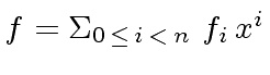 .
In order to evaluate
.
In order to evaluate ![]() at
at
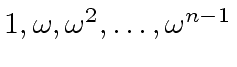 ,
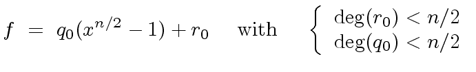
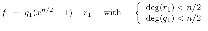
we follow a divide-and-conquer strategy; more precisely, we consider
the divisions with remainder of
,
we follow a divide-and-conquer strategy; more precisely, we consider
the divisions with remainder of ![]() by
by
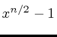 and
and
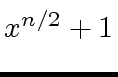 .
So let
.
So let
 be polynomials such that
 and
and
 hold because the polynomial
  and
and
 can be done very easily.
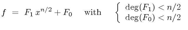
Indeed, let
can be done very easily.
Indeed, let
![$ F_0, F_1 \in R[x]$](img185.png) be such that
be such that
 |
(33) |
 |
(34) |
 |
(35) |
 .
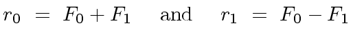
By using Relation (31) with
.
By using Relation (31) with
 |
(36) |
 |
(37) |
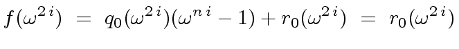
 .
Indeed, this last equation follows from
.
Indeed, this last equation follows from
 |
(38) |
 is not zero
nor a zero divisor.
Therefore we have proved the following
is not zero
nor a zero divisor.
Therefore we have proved the following
![$ f \in R[x]$](img198.png) (with degree less than
(with degree less than  is equivalent to
, and
.
is equivalent to
, and
.
 -th root of unity
we can hope for a recursive algorithm.
This algorithm would be easier if both
-th root of unity
we can hope for a recursive algorithm.
This algorithm would be easier if both  |
(39) |
be a primitive  using
using
 additions in
  multiplications by powers of
  ring operations.
 .
Let
.
Let  and
and  be the number of additions
and multiplications in
be the number of additions
and multiplications in  whose costs is null
thus we have
whose costs is null
thus we have  and
and  which satisfies
the formula since
which satisfies
the formula since
 .
Assume
.
Assume  .
Just by looking at the algorithm we that
.
Just by looking at the algorithm we that
 |
(40) |
![\fbox{
\begin{minipage}{10 cm}
\begin{description}
\item[{\bf Input:}] $n = 2^k$...
...({\omega}^{n-2}), r_1^{\ast}({\omega}^{n-2}))$\ \\
\end{tabbing}\end{minipage}}](img207.png)