Proof.
Let
(
a0,
a1,...,
ad) be a
p-adic expansion of
a w.r.t.
p.
Let
k <
d + 1 be a positive integer.
By Proposition
13,
the element
| a(k) = a0 + a1p + ... ak-1pk-1 |
(92) |
is a
p-adic approximation of
a at order
k.
By Proposition
11
there exists a polynomial

 R
R[
y] such that
 (a(k) + akpk) = (a(k)) + (a(k) + akpk) = (a(k)) +  (a(k))akpk + (a(k))akpk +  (a(k) + akpk)(akpk)2. (a(k) + akpk)(akpk)2. |
(93) |
Since we have
a  a(k) + akpkmodpk+1 a(k) + akpkmodpk+1 |
|
we deduce from Proposition
14
| (a) (a(k) + akpk)modpk+1 |
(94) |
Since

(
a) = 0 this shows that
(
a(k) +
akpk) is in the ideal generated by
pk+1.
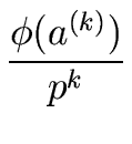
Similarly,
(
a(k)) is in the ideal generated by
pk.
Therefore we can divide
(
a(k) +
akpk) and
(
a(k)) by
pk, leading to
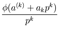 = =  + (a(k))ak + (a(k) + akpk)(ak)2pk. + (a(k))ak + (a(k) + akpk)(ak)2pk. |
(95) |
Now observe that
| 0 (a(k) + akpk)(ak)2pkmodp. |
(96) |
Let us denote by

the canonical homomorphism from
R to
R/
 p
p
.
Then we obtain
Now, since
a  a0
a0mod
p holds we have
Finally, since
(
a0)

0 mod
p holds we can solve
Equatiion
97
for
(
ak).

Theorem 13
Let
R be a commutative ring with identity element
and let

be a finitely generated ideal of
R.
Let
r be a positive integer.
Let
f1,...,
fn R[
x1,...,
xr] be
n
multivariate polynomials in the
r variables
x1,...,
xr.
Let
a1,...,
ar R be elements.
Let
U be the Jacobian matrix of
f1,...,
fn
evaluated at
(
a1,...,
ar).
That is,
U is the
n×
r matrix defined by
U = (uij) where uij =  (a1,..., ar) (a1,..., ar) |
(99) |
We assume that the following properties hold
- for every
i = 1 ... n we have
fi(a1,..., ar) 0 mod.
- the Jacobian matrix U is left-invertible.
Then, for every positive integer

we can compute
a( )1
)1,...,
a()r R such that
- for every
i = 1,..., n we have
fi(a()1,..., a()r) 0 mod,
- for every
j = 1,..., r we have
a()j ajmod.
Proof.
We proceed by induction on

1.
For
= 1 the claim follows from the hypothesis of the theorem.
So let
1 be such that the claim is true.
Hence there exist
a()1,...,
a()r R such that
fi(a()1,..., a()r) 0 mod , i = 1,..., n , i = 1,..., n |
(100) |
and
| a()j ajmod, i = 1,..., r |
(101) |
Since
is finitely generated, then so is
and let
g1,...,
gs R such that
Therefore, for every
i = 1,...,
n, there exist
qi1,...
qis R
such that
fi(a()1,..., a()r) =  qikgk qikgk |
(103) |
For each
j = 1,...,
r we want to compute
Bj R such that
| a(+1)j = a()j + Bj |
(104) |
is the desired
next approximation.
We impose
Bj so let
bj1,...,
bjs R be such that
| Bj = bjkgk |
(105) |
Using Proposition
12
we obtain
where
 u()ij
u()ij
is the Jacobian matrix
of
(
f1,...,
fn) at
(
a()1,...,
a()r).
Hence, solving for
a(+1)1,..., a(+1)r R
such that
| fi(a(+1)1,..., a(+1)r) 0 mod+1 |
|
leads to solving the system of linear equations:
qik +  u()ijbjk 0 mod u()ijbjk 0 mod |
(107) |
for
k = 1,...,
s and
i = 1,...,
n.
Now using
a()j ajmod
for
j = 1,..., r we obtain
Therefore the system linear equations
given by Relation (
107)
has solutions.
 (
(