Greatest Common Divisors and Primes
Contents
4.2. Greatest Common Divisors and Primes#
Greatest common divisors (GCDs) and prime numbers are a fundamental part of number theory. They have been extensively studied for thousands of years. Euclid was fundamental to the study of prime numbers and number theory. As we will see, Euclidean division extends to the Euclidean algorithm for computing GCDs.
4.2.1. Prime numbers#
Definition (prime)
An integer \(p > 1\) is prime if the only divisors of \(p\) are \(1\) and \(p\). An integer which is not prime is called composite.
For example, \(7\) is prime because only \(1\) and \(7\) divide \(7\). On the other hand, \(3\) divides \(9\), and so \(9\) is not prime.
Recall that another way of describing divisors is as factors. Therefore, an equivalent definition of a prime number \(p\) is one whose factors are only 1 and \(p\).
The fundamental theorem of arithmetic strengthens the idea of primality to a prime factorization.
Theorem 4.2.1 (fundamental theorem of arithmetic)
Every integer greater than \(1\) is either prime or can be written as the product of two or more primes.
Formally, the theorem can be stated as follows. For every integer \(c > 1\), there exists a positive integer \(n\), prime numbers \(p_1, \ldots, p_n\), and exponents \(e_1, \ldots, e_n\) such that:
This theorem is also called the unique factorization theorem. It tells us that any number which is not prime is the product of some primes.
Prime factorization
The following are prime factorizations.
\(6 = 2 \cdot 3\)
\(16 = 2\cdot 2\cdot 2\cdot 2 = 2^4\)
\(42 = 2\cdot 3\cdot 7 \)
\(1234 = 2 \cdot 617\)
\(1008 = 2 \cdot 2 \cdot 2 \cdot 2 \cdot 3 \cdot 3 \cdot 7 = 2^4 \cdot 3^2 \cdot 7\)
Since multiplication is commutative, prime factorization is only unique up to the ordering of factors.
To get a unique prime factorization, we often add an additional constraint to the fundamental theorem of arithmetic. This constraint requires the primes to listed in increasing order: \(p_1 < p_2 < \cdots < p_n\).
4.2.2. Finding Primes#
How can we determine if a number is prime?
A simple and brute-force solution is to try and divide the number in question by every other integer less than it. If there are no divisors, then the number is prime. This method by “trial division” is very inefficient.
The sieve of Eratosthenes is a more efficient method. It is based on the following observation.
Proposition 4.2.2
If a positive integer \(n\) is composite, then it must have a prime divisor less than or equal to \(\sqrt{n}\)
Proof: If \(n\) is a positive composite then there exists two integers \(a, b\) greater than 1 such that \(n = ab\). Certainly \(a \leq \sqrt{n}\) or \(b \leq \sqrt{n}\). If \(n\) is a perfect square then \(a = b = \sqrt{n}\). Otherwise, one of \(a\) or \(b\) must be smaller than \(\sqrt{n}\).
The sieve of Eratosthenes uses this proposition to remove all composite numbers from a list and retain only the prime ones.
The sieve of Eratosthenes
Let \(S = \{2, 3, \ldots, 100\}\). Since the maximum element of \(S\) is \(100\), we only need to consider primes divisors less than \(\sqrt{100} = 10\).
Find the smallest element of \(S\). This is \(2\). This element is prime. Remove from \(S\) all multiples of \(2\) other than \(2\) itself.
Find the next smallest element of the remaining numbers. This is \(3\). Remove from \(S\) all multiples of \(3\) other than \(3\) itself.
Find the next smallest element of the remaining numbers. This is \(5\). Remove from \(S\) all multiples of \(5\) other than \(5\) itself.
Find the next smallest element of the remaining numbers. This is \(7\). Remove from \(S\) all multiples of \(7\) other than \(7\) itself.
The next smallest element of \(S\) is 11. Since \(11 > 10\), we can stop. Every remaining number is prime.
The prime numbers less than 100 are:
4.2.3. Computing Primes#
Finding and, in particular, generating primes is a very practical problem. A large class of digital security and cryptography algorithms rely on prime numbers.
However, there is no known closed form formula or function which always produces primes. For example, the function \(f(n) = n^2 - n + 41\) results in prime numbers for all choices of \(n\) between \(1\) and \(40\). However, \(f(41) = 41^2\) is not prime.
On the other hand, we do know that there are infinitely many primes, so we can always find primes, with enough effort.
Theorem 4.2.3
There are infinitely many prime numbers.
Proof
Proceed by contradiction and assume that there are finitely many primes: \(p_1, p_2, \ldots, p_n\). Let \(q = p_1p_2\cdots p_n + 1\).
By the fundamental theorem of arithmetic, \(q\) is either prime or a product of primes. If \(q\) is prime then we have a contradiction where \(p_1, p_2, \ldots, p_n\) cannot be the list of all primes since \(q\) is not in that list and is prime.
On the other hand, consider if \(q\) is a product of primes. Let \(p_j\) be such a prime divisor of \(q\). That is, \(p_j \mid p_1p_2\cdots p_n + 1\). However, we also have \(p_j \mid p_1p_2\cdots p_n\). Therefore, it must be that \(p_j \mid q - p_1p_2\cdots p_n\), that is, \(p_j \mid 1\). However, this is not possible since every prime is greater than \(1\). This is a contradiction.
In either case we have that \(p_1, p_2, \ldots, p_n\) cannot possibly be the list of all primes. Hence, there are infinitely many primes. \(\blacksquare\)
Even though there are infinitely many primes, actually generating them is a challenge. By trial division or the sieve of Eratosthenes, we can determine if a number is prime. However, for large numbers, this is very inefficient.
Another test of primality is based on Fermat’s little theorem.
Theorem 4.2.4 (Fermat’s little theorem)
For two positive integers \(a\) and \(p\), if \(p\) is prime and \(p \nmid a\), then:
Proof
Nope! This proof is well beyond the scope of this course. See wikipedia.
For example, we know that \(5\) is prime and \(5 \nmid 16\). By Fermat’s little theorem, it must be that \(16^4 \equiv 1 \bmod 5\). Indeed, we have \(16^4 = {2^4}^4 = 2^{16} = 65536\) and \(65536 \equiv 1 \bmod 5\).
Fermat’s little theorem gives rise to the Fermat primality test. Given some positive integer \(n\), we can deduce that \(n\) is not prime if we can find a number \(a\) such that \(a^{n-1} \not\equiv 1 \bmod n\). Such an \(a\) is called a Fermat witness.
The Fermat primality test leads to a probabilistic method to determine if a number is prime. A probabilistic algorithm is one which produces the correct result “with high probability” but not necessarily all of the time.
For primality, the probabilistic method tries to find a Fermat witness. If, after a certain number of attempts, it cannot find such a witness, then the algorithm terminates and assumes that the number is prime. This assumption is what makes the algorithm probabilistic. Only if we compute \(a^{p-1}\) for every \(1 < a < n\) will we know for certain that \(n\) is prime.
How many times should we try to find a Fermat witness before giving up? The answer is not clear. Computing the exact probability of error is challenging. Qualitatively, the more attempts we make to find a Fermat witness, the better chance there is that \(n\) is actually prime. Hence, one can feel “good” if they try a “reasonably large” number of times to find a Fermat witness. Maybe 100? 256? 1000? It depends on how long you are willing to wait and how large your candidate number is.
The below Python code implements the Fermat primality test by choosing random integers \(a\) as possible Fermat witnesses. It generates random primes by choosing using this test.
from random import randint

def isPrime(p, numIter) :
    for i in range(numIter) :
        a = randint(2, p-1)
        e = a**(p-1) % p #this is *very* inefficient
        if (e != 1) :
        	return False
    return True

def randomPrime(n) :
    while(True) :
	    p = randint(2**(n-1), 2**(n)-1)
	    if isPrime(p, 128) :
	    	return p;

#print a random 32-bit prime
print(randomPrime(16))
49103
Prime Conjectures
Primes have been studied for thousands of years by countless researchers. Yet, many properties have still been unproved. The following are conjectures many believe to be true.
Goldbach’s conjecture: Every even integer \(n\) greater than \(2\) is the sum of two primes. This has been verified for numbers up to \(1600000000000000000\) (\(1.6 \times 10^{18}\)).
Landau’s conjecture: There are infinitely many primes of the form \(n^2 + 1\), for a positive integer \(n\). On the other hand, it has been proven that there are infinitely many composite numbers of the form \(n^2 + 1\). But, this does not disprove Landau’s conjecture.
Twin Prime conjecture: There are infinitely many primes that differ by \(2\). Twin primes include \(5\) and \(7\), \(11\) and \(13\), \(71\) and \(73\), etc.
4.2.4. Greatest Common Divisors#
Definition (greatest common divisor)
For two non-zero integers \(a\) and \(b\), \(d\) is the greatest common divisor of \(a\) and \(b\) if \(d \mid a\), \(d \mid b\), and any other common divisor of \(a\) and \(b\) also divides \(d\).
For small numbers, it is easy to compute GCDs by eye.
For example, a GCD of \(12\) and \(18\) is \(6\). Yet, another GCD of \(12\) and \(18\) is \(-6\). Consider the again the definition of GCD. The common divisors of \(12\) and \(18\) are \(-2\), \(-3\), \(-6\), \(2\), \(3\), and \(6\). Since \(\pm 2\), \(\pm 3\) and \(6\) all divide \(-6\), and \(\pm 2\), \(\pm 3\), and \(-6\) all divide \(6\), both \(6\) and \(-6\) are GCDs of \(12\) and \(18\).
To make life easier, we typically decide on a “canonical” GCD and call it the GCD. For the integers, the canonical GCD is the positive one. Therefore, the GCD of \(12\) and \(18\) is \(6\).
We can write the GCD of two numbers in a functional notation. For example, \(\gcd(12,18) = 6\).
Definition (relatively prime)
Two integers are relatively prime if their greatest common divisor is \(1\). We call two such integers co-prime.
Every pair of numbers has a trivial common divisor: \(1\). When two numbers have a GCD that is greater than \(1\), we say they have a non-trivial GCD. Otherwise, they are relatively prime. That means, they do not share any common factors.
When we have a collection of integers, we say that they are pairwise relatively prime if every integer in the collection is relatively prime to every other integer. That is, for integers \(a_1, a_2, \ldots, a_n\), we have \(\gcd(a_i, a_j) = 1\) for \(1 \leq i < j \leq n\).
We can determine the GCD of two numbers, or if they are relatively prime, based on their prime factorizations.
If any of the primes \(p_i\) equals a prime \(q_j\), then \(a\) and \(b\) have a non-trivial GCD. If \(a\) and \(b\) have no primes in common between their prime factorizations, then they are relatively prime.
We can compute the GCD of \(a\) and \(b\) from their prime factorization by getting the product of all common primes raised the minimum exponent of that prime in either number.
Computing GCDs from primes
We compute the GCD of \(1470\) and \(350\).
The GCD of \(1470\) and \(350\) is thus \(2^{\min{(1,1)}} \cdot 5^{\min{(1,2)}} \cdot 7^{\min{(2,1)}} = 70\).
Least Common Multiples#
We can also use prime factorization to compute the least common multiple (LCM) between two integers.
Definition (least common multiple)
The least common multiple of two positive integers \(a\) and \(b\) is the smallest positive integer that is divisible by both \(a\) and \(b\).
Whereas we computed the GCD by taking the common primes of two integers (i.e. the intersection of primes in their factorization), we compute the LCM by taking the union of primes in their factorization. Then, each prime is raised to the maximum exponent of that prime in either number.
Computing LCMs from primes
We compute the LCM of \(1470\) and \(350\).
The LCM of \(1470\) and \(350\) is thus \(2^{\max{(1,1)}} \cdot 3^{\max{(1,0)}} \cdot 5^{\max{(1,2)}} \cdot 7^{\max{(2,1)}} = 7350\).
While this method is easy by inspection, computing the prime factorization of number, in general, is very hard. Therefore, this method is not practical. A more practical method is the Euclidean algorithm which we will study shortly.
Before that, we conclude with a theorem. Can you prove it?
Theorem 4.2.5
For any two positive integers \(a\) and \(b\), we have:
Euclidean Algorithm#
The Euclidean algorithm is an efficient method for computing the GCD of two integers. As can be inferred from its name, the algorithm has been known for many centuries and can be attributed to Euclid. The algorithm is based on a simple idea rooted in Euclidean division.
Let \(a = bq + r\) by Euclidean division. Then, \(r = a - bq\). Now, let \(d\) be a common divisor of \(a\) and \(b\). That is, \(d \mid a\) and \(d \mid b\). Certainly, then, we have \(d \mid r\) since \(r = a - bq\).
In summary, we have the following lemma.
Lemma 4.2.6
Let \(a\) and \(b\) be integers with \(a = bq + r\) by Euclidean division. Thus, \(0 \leq r < b\). We have:
Therefore, the foundation of the Euclidean algorithm is repeated applications of Euclidean division.
Euclidean by example
Let us find the GCD of \(287\) and \(91\) by the Euclidean algorithm.
\(287 = 91\cdot 3 + 14\). That is, \(287\) mod \(91\) = 14.
\(91 = 14\cdot 6 + 7\). That is, \(91\) mod \(14\) = 7.
\(14 = 7\cdot 2 + 0\). That is, \(14\) mod \(7\) = 0.
Since we cannot divide by 0 in the next step, the process terminates and we have:
This previous example results in a remainder sequence starting at \(287\) and ending at \(0\):
We can verify that \(7\) is a common divisor at every step. \(7 \mid 0\), \(7 \mid 7\), \(7 \mid 14\), \(7 \mid 91\), and \(7 \mid 287\). This is as expected from the previous lemma.
Moreover, notice that this remainder sequence is strictly decreasing. From Euclidean division we have \(a = bq + r\) with \(0 \leq r < b\). Since the magnitude of successive remainders strictly decreases, and has \(0\) as a lower bound, it must be that repeated applications of Euclidean division will lead to a \(0\) remainder and thus termination of the algorithm. The correctness follows from the previous lemma.
Finally, we state the algorithm. Its termination and correctness is guaranteed by the previous discussion.
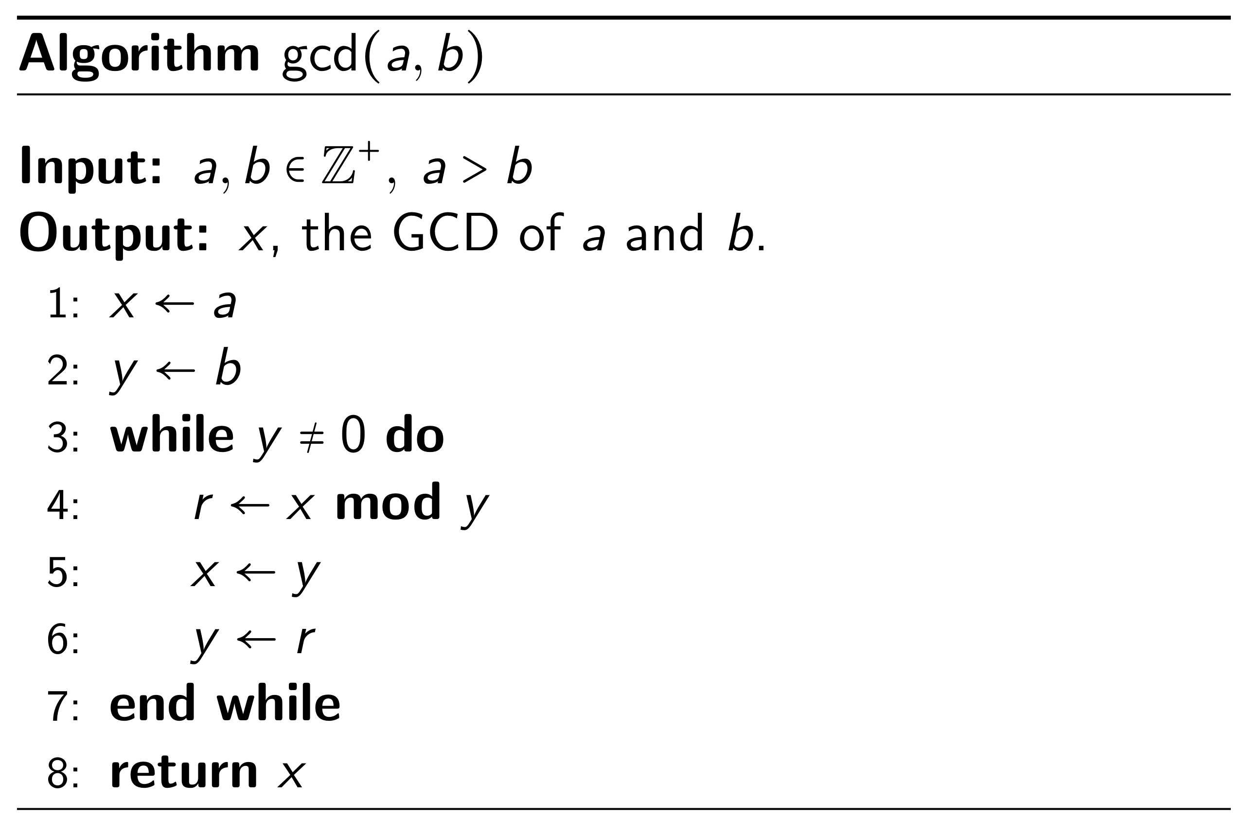
We can also see the Euclidean algorithm in action in Python.
def gcd(a,b) :
    x = a
    y = b
    print("r0: %d" % x)
    print("r1: %d" % y)
    i = 2;
    while y != 0 :
        r = x % y
        print("r%d: %d" % (i, r))
        i += 1
        x = y
        y = r
    return x

print("GCD(152152, 154700) = %d" % gcd(152152, 154700))
r0: 152152
r1: 154700
r2: 152152
r3: 2548
r4: 1820
r5: 728
r6: 364
r7: 0
GCD(152152, 154700) = 364
Bézout Relations and GCDs#
An interesting property of GCDs is that they can be written as a linear combination of the two input integers.
Theorem 4.2.7 (Bézout’s theorem)
For any positive integers \(a\) and \(b\), there exists integers \(s\) and \(t\) such that:
From this theorem we extract some definitions. The formulas \(\gcd(a,b) = sa + sb\) is called the Bézout identity. The integers \(s\) and \(t\) are called the Bézout coefficients of \(a\) and \(b\).
A first Bézout relation
The Bézout coefficients of \(6\) and \(14\) are \(-2\) and \(1\).
We can find the Bézout coefficients of two numbers through a “two pass” method using the Euclidean algorithm. Consider the Euclidean algorithm executed on \(252\) and \(198\).
Therefore, \(\gcd(252,198) = 18\). Now, how can we write \(18\) as a combination of \(252\) and \(198\)? We can work bottom-up from the successive Euclidean divisions and back-substitute one equation at a time.
The first line comes from \(54 = 1 \cdot 36 + 18\). The second line comes from \(198 = 3 \cdot 54 + 26\) substituted into the previous. The third line comes from \(252 = 1\cdot 198 + 54\) substituted into the previous.
This two-pass method is sufficient for computations by hand. However, a more efficient method is to compute a sequence of Bézout coefficients at each step of the algorithm. Alongside the sequence of remainders \((r_i)\), one also computes a sequence of Bézout coefficients \((s_i)\) and \((t_i)\). These sequences start as:
See more about the Extended Euclidean Algorithm here.
Consequences of Bézout#
Lemma 4.2.8
Let \(a, b, c\) be positive integers such that \(a\) and \(b\) are relatively prime. If \(a \mid bc\) then \(a \mid c\).
Proof:
Since \(a\) and \(b\) are relatively prime, we have \(\gcd(a,b) = 1\). By hypothesis assume \(a \mid bc\).
By Bézout’s theorem, we have \(sa + tb = \gcd(a,b) = 1\). Then, multiply both by \(c\) to get: \(csa + ctb = c\). Since \(a \mid bc\), \(a \mid ctb\). That is, there exists \(q\) such that \(ctb = qa\).
Therefore, we have:
Hence, \(a \mid c\), as required. \(\blacksquare\)
This lemma can be generalized for prime and composite numbers.
Lemma 4.2.9
Let \(p\) be a prime integer and \(a_1, a_2, \ldots, a_n\) be integers.
If \(p \mid a_1a_2\cdots a_n\), then \(p \mid a_i\) for at least one \(i\).
We saw earlier in Congruence, sums, and products that division did not always maintain congruence relations. However, with Bézout relations we can describe when divisions do maintain congruence.
Theorem 4.2.10
Let \(m\) be a positive integer and \(a,b,c\) be integers.
If \(\gcd(c,m) = 1\) and \(ac \equiv bc \bmod m\), then \(a \equiv b \bmod m\).
Proof:
By the hypothesis we have \(ac \equiv bc \bmod m\), hence:
From the previous lemma, \(m\) must therefore divide \(c\) or \((a-b)\). Since, by assumption, \(\gcd(c,m) = 1\), it must be that \(m \mid a-b\). That is, \(a \equiv b \bmod m\). \(\blacksquare\)
4.2.5. Exercises#
Exercise 4.10
Write a Python function that takes an integer \(n\) and prints all prime numbers between \(2\) and \(n\). Use the sieve of Eratosthenes as your algorithm.
Exercise 4.11
Determine the following values.
\(\gcd(-24, 18)\)
\(\gcd(756, 210)\)
\(\gcd(-756, 210)\)
\(\gcd(742, 14)\)
Solution to Exercise 4.11
6
42
42
14
Exercise 4.12
Compute the prime factorization of the following numbers.
\(78\)
\(672\)
\(7920\)
Solution to Exercise 4.12
\(2 \cdot 3 \cdot 13\)
\(2^5 \cdot 3 \cdot 7\)
\(2^4 \cdot 3^2 \cdot 5 \cdot 11\)
Exercise 4.13
Let \(A = \{x \in \mathbb{Z} \ |\ 1 \leq x \leq 10\}\). Let \(\mathcal{R}\) be a binary relation on \(A\) where \(a\mathcal{R}b\) if \(a \mid b\).
Draw a Hasse diagram for \(\mathcal{R}\).
Exercise 4.14
Prove the following statement.
Proposition
Let \(a\) be an integer. \(a^2 - 2\) is never divisible by \(4\).
Solution to Exercise 4.14
Proceed by contradiction. Assume \(4 \mid a^2 - 2\). Then, \(\exists q \in \mathbb{Z}\) such that \(4q = a^2 - 2\).
Assume \(a\) is even. Then \(a = 2x\) for some integer \(x\), and:
which says \(4 \mid 2\), which is not possible.
Assume \(a\) is odd. Then \(a = 2x + 1\) for some integer \(x\), and:
which says \(4 \mid 1\), which is impossible.
Therefore, \(4 \nmid a^2 - 2\) for any integer \(a\).
Exercise 4.15
Prove the following statement.
Proposition
Let \(n\) be a natural number and \(x\) be an integer. In the sequence of \(n\) consecutive integers \(x, x+1, x+2, \ldots, x+n-1\), at least one of them is divisible by \(n\).
Solution to Exercise 4.15
By Euclidean division we have \(x = nq + r\) with \(0 \leq r < n\).
If \(r = 0\), then \(x = nq\) and \(n \mid x\). If \(r = 1\), then \(x = nq + 1\), \(x + n - 1 = n(q+1)\) and \(n \mid x + n -1\). If \(r = 2\), then \(x = nq + 2\) and \(n \mid x + n -2\). Continuing, if \(r = k\) then \(x = nq + k\) and \(n \mid x + n -k\).
Since \(0 \leq r < n\) ranges over \(n\) consecutive values, it covers all cases of \(x, x+1, \ldots, x+n-1\).
Exercise 4.16
RSA is a cryptography system which relies of exponentiation and modular numbers. In particular, it is relatively easy to find three integers \(e,d,m\) such that, for any integer \(n\), \(0 \leq n < m\),
We call \(n^e\) the encrypted message and \(e\) the public key. Then, \((n^e)^d \equiv n\) is the decrypted message and \(d\) is the private key.
In particular, we can compute such an \(m\) as the least common multiple of \(p-1\) and \(q-1\) for two different prime numbers \(p\) and \(q\). If \(p = 7\) and \(q = 11\) then \(m= 30\).
Find \(e\) and \(d\) such that \((3^e)^d \equiv 3 \bmod 30\).
Tip: use a calculator or python to handle the big numbers!
Solution to Exercise 4.16
Any two numbers which are multiplicative inverses modulo 30 will work. For example, 7 and 13, 11 nad 11, 17 and 23, 19 and 19, 29 and 29.